Short Version

Ohm’s Law:

$v = iR$

Resistors in series:

$R_{eq} = R_1 + R_2 + R_3$

Resistors in parallel:

$\frac{1}{R_{eq}} = \frac{1}{R_1} + \frac{1}{R_2} + \frac{1}{R_3}$

Two resistors in parallel:

$R_{eq} = \frac{R_1R_2}{R_1 + R_2}$

The derivative (i.e. rate of change) of inductor current is proportional to the voltage:

$v = L\frac{di}{dt}$

Inductors in series:

$L_{eq} = L_1 + L_2 + L_3$

Inductors in parallel:

$\frac{1}{L_{eq}} = \frac{1}{L_1} + \frac{1}{L_2} + \frac{1}{L_3}$

Two inductors in parallel:

$L_{eq} = \frac{L_1L_2}{L_1 + L_2}$

The derivative (i.e. rate of change) of capacitor voltage is proportional to the current:

$i = C\frac{dv}{dt}$

Capacitors in series (note difference between this and resistors/inductors in series):

$\frac{1}{C_{eq}} = \frac{1}{C_1} + \frac{1}{C_2} + \frac{1}{C_3}$

Capacitors in parallel (note different between this and resistors/inductors in parallel):

$C_{eq} = C_1 + C_2 + C_3$

Angular frequency $\omega$ in radians per second is prortional to frequency f in Hertz (cycles per second):

$\omega = 2 \pi f$

Impedance is a bit like complex-valued resistance. It comprises a real part (resistance R) and an imaginary part (reactance X):

$Z = R + jX$

where the reactance X is generally a function of frequency.

Resistors are purely resistive. The impedance of a resistor is just equal to its resistance:

$Z_R = R + 0j = R$

Inductors are purely reactive. The reactance of an inductor is

$X_L = \omega L$

Note that the reactance of an inductor is always positive.

The impedance of an inductor is purely imaginary:

$Z_L = 0 + jX_L = j \omega L$

Capacitors are purely reactive. The reactance of a capacitor is

$X_C = \frac{-1}{\omega C}$

Note that the reactance of a capacitor is always negative.

The impedance of a capacitor is purely imaginary:

$Z_C = 0 + jX_C = \frac{1}{j \omega C} = \frac{-j}{\omega C}$

AC networks are often analysed using phasors. A phasor is a complex value which represents a sinusoidal voltage or current. The magnitude of the phasor’s complex value represents the magnitude of the AC voltage or current (normally the r.m.s. value). The angle of the phasor’s complex value represents the phase difference between the voltage or current and the reference phasor. In principle, any voltage or current phasor in the network can be chosen as the reference. In practice however, the voltage source driving the network reference phasor is often selected as the reference phasor.

A sinusoidal AC voltage can be represented using an expression of the following form:

$v(t) = V_p \cos\left(\omega t + \phi \right)$

where $V_p$ is the peak voltage, $\omega$ is the angular frequency (rad/s) and $\phi$ is the phase angle of the voltage.

It is often convenient to express the magnitude of an AC voltage or current as an r.m.s. (root mean square) value. For sinusoidal signals, the r.m.s. magnitude is simply the peak value divided by $\sqrt{2}$ . For example, the AC voltage $v(t)$ defined above has a peak value of $V_P$ . Its corresponding r.m.s. voltage is

$V_{rms} = \frac{V_p}{\sqrt{2}}$

The above expression for v(t) can therefore be stated equivalently as

$v(t) = \sqrt{2}V_{rms}\cos \left( \omega t + \phi \right)$

Phasor analysis is underpinned by the use of imaginary exponents to represent sinusoidal variation. Euler’s Formula states

$e^{j\theta} = \cos(\theta) + j\sin(\theta)$

where e is Euler’s number (approximately 2.71828), j is the square root of $-1$ , and $\theta$ is an angle in radians.

Suppose the angle $\theta$ is not a constant value, but a function of time:

$e^{j\omega t} = \cos \left(\omega t\right) + j \sin\left( \omega t \right)$

This is the basic building block of phasor analysis. A phasor is basically just a complex number that you multiply $e^{j \omega t}$ by to adjust its magnitude and angle to match a particular voltage or current in an AC circuit.

Note that the real part of the above expression is

$\mathrm{Re}\left( e^{j \omega t} \right) = \cos \left( \omega t \right)$

which is just a sinusoidal signal with angular frequency $\omega$ and amplitude equal to 1.

If $V_1$ is a complex-valued voltage phasor, the time domain voltage function it represents is

$v_1(t) = \mathrm{Re}\left( V_1 e^{j \omega t} \right)$

Representing $V_1$ in polar form,

$v_1(t) = \mathrm{Re}\left( \left| V_1 \right| e^{j \angle{V_1}} e^{j \omega t} \right)$

Bearing in mind the following property of exponents: $x^a \times x^b = x^{a+b}$ ,

$v_1(t) = \mathrm{Re}\left( \left| V_1 \right| e^{j \left(\omega t + \angle{V_1}\right)} \right)$

Therefore,

$v_1(t) = \left| V_1 \right| \cos\left( \omega t + \angle{V_1}\right)$

where $|V_1|$ and $\angle V_1$ are the magnitude and angle of the complex number $V_1$ respectively.

Note that:

The magnitude of the phasor has scaled the magnitude of the cosine function.
The angle of the phasor has shifted the phase of the cosine function.

Remember: In phasor analysis of AC circuits, it is assumed that all voltages and currents are sinusoidal and have the same frequency. A phasor is just a complex number, which provides a handy way of storing and manipulating the two other two parameters of each sinusoidal signal: amplitude and phase.

r.m.s. phasors

The magnitude of a phasor can either represent the peak value of a voltage or current, or it can represent the r.m.s. value. When analysing electrical power systems, it is far more common for phasors to represent r.m.s. values of voltage and current because that greatly simplifies the calculation of power values in the network. For this reason, all further discussion below assumes that phasors represent r.m.s. values. Furthermore, all phasors featured in the exam will represent r.m.s. values!

If $V_a$ is a complex-valued r.m.s. voltage phasor, the time domain voltage it represents is

$v_1(t) = \left| V_a \right| \sqrt{2} \cos\left( \omega t + \angle{V_a}\right)$

where $|V_a|$ and $\angle V_a$ are the magnitude and angle of complex number $V_a$ respectively.

The formula relating voltage phasor V and current phasor I in a circuit with impedance Z is very similar to Ohm’s Law:

$V = IZ$

In fact, when using phasors to analyse networks of impedances driven by AC voltage and current sources, we can apply most of the same techniques that are used to anaylse resistive networks driven by DC sources. However, since impedances are complex values, all calculations must be carried out using complex arithmetic.

Impedances in series:

$Z_{eq} = Z_1 + Z_2 + Z_3$

Impedances in parallel:

$\frac{1}{Z_{eq}} = \frac{1}{Z_1} + \frac{1}{Z_2} + \frac{1}{Z_3}$

Two impedances in parallel? Remember…

ZIPPOS: Zs In Parallel? Product Over Sum!

$Z_{eq} = \frac{Z_1Z_2}{Z_1 + Z_2}$

A very useful acronym:

CIVIL

In a capacitor (C), current (I) leads voltage (V).
Voltage (V) leads current (I) in an inductor (L).

Some other techniques which can be used in phasor analysis of impedance networks (provided that you use complex arithmetic throughout):

Superposition for analysing AC networks with more than one source. (Note: All sources must have the same frequency.)
Thevenin and Norton equivalent circuits.
Star-delta transformations.

Phasors and Power

Recall that instantaneous power in a circuit is given by

$p = vi$

where v is the voltage in volts (V) and i is the current in amperes (A). The unit of instantaneous power is the watt ( W ).

In a DC circuit where voltage and current are constant, the average power is exactly the same as the instantaneous power.

The situation in AC circuits is more complicated because in general there is a phase difference between current and voltage.

We talk about four kinds of power in AC circuits:

complex power, S
active power, P
reactive power, Q
apparent power, |S|

The complex power, S, is the product of r.m.s. phasors V and I^* (that’s the complex conjugate of the current phasor):

$S = VI^*$

The unit of complex power is the volt-ampere.

The active power, P, is the real part of S.

$P = \mathrm{Re}\left( VI^* \right)$

Since inductors and capacitors are purely reactive, they cannot dissipate real power. In RLC circuits, the active power is therefore the sum of power dissipated as heat in all resistors. Because active power is real power, and represents the use of electrical energy to do work, the unit of active power is the watt ( W ).

Please remember: Inductors and capacitors cannot dissipate active (real) power. All active power in RLC circuits must be dissipated in resistors!

The power factor is the cosine of $\phi$ , the phase difference between current and voltage in the circuit. It is given this name because of the following relationship:

$P = |V||I| \cos( \phi )$

where |V| and |I| are the magnitudes of complex-valued r.m.s. phasors V and I and $\phi = \angle V - \angle I$ . Since the power factor is the cosine of an angle, it is dimensionless (it has no units).

The reactive power, Q, is the imaginary part of S.

$Q = \mathrm{Im}\left( VI^* \right) = |V||I| \sin ( \phi )$

where V and I are the complex-valued phasors representing voltage and current in the circuit and $\phi = \angle V - \angle I$ , i.e. the phase difference between V and I. The unit of reactive power is the volt-ampere reactive (var) – note that this unit name is correctly written in lower case.

The final power value is apparent power, simply denoted by |S|, which is the product of the magnitudes of the voltage and current in the circuit.

$|S| = |V||I|$

The unit of apparent power is the volt-ampere (VA). Apparent power can be thought of as the power that would be dissipated in the circuit if the current and voltage were perfectly in phase, i.e. if $\phi = \angle V - \angle I = 0$ .

In purely resistive circuits, voltage and current are always in phase, so S is real and $P = |S| = S$ .
In RLC circuits, AC voltage and current are not generally in phase, so S is complex and $P \leq |S|$ .

Transients in DC circuits

When an RC circuit responds to a step change in input voltage, the time is takes to move 63.2% of the way to its new steady state voltage is known as the time constant, $\tau$ . The value of $\tau$ for an RC circuit is

$\tau = RC$

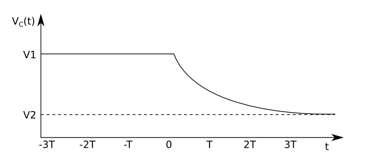
If the capacitor voltage is $v_C(t) = V_1$ for $t<0$ , begins changing at $t=0$ , and $v_c(t) \to V_2$ as $t \to \infty$ , the complete transient response of the capacitor voltage is described by

$v_C(t) = V_2 - (V_2-V_1).e^{\frac{-t}{\tau}}$

That equation will work for transient changes in $v_c$ between any starting voltage $V_1$ and finishing voltage $V_2$ . However, in many cases, either $V_1$ or $V_2$ is zero, in which case the formula is simplified slighly:

When the capacitor begins completely discharged, i.e. $V_1 = 0$ , and the capacitor is charging up to a voltage $V_2 = V_S$ with time constant $\tau = RC$ ,

$v_c(t) = V_S.\left( 1 - e^{\frac{-t}{\tau}} \right)$

When the capacitor begins the transient with a voltage on it (e.g. $V_1 = V_S$ ) and discharges down to $V_2 = 0$ with a time constant $\tau = RC$ ,

$v_c(t) = V_S.e^{\frac{-t}{\tau}}$

Example

Let’s say that $V_1 = 5 \mathrm{V}$ and $V_2 = 0 \mathrm{V}$ ,

$v_C(t) = 5.\left( 1 - e^{\frac{-t}{\tau}} \right)$

Note that the significance of the 63.2% value is that $1 - e^{-1} = 0.6321$ .

For example, using the values of $V_1$ and $V_2$ specified above, at time $t = \tau$ ,

$v_C(\tau) = 5.\left( 1 - e^{-1} \right) = 0.6321 \times 5 \mathrm{V}$

The concept of a time constant can be applied to many different systems or process that exhibit exponential decay, including for example heating and cooling of a building, or radioactive decay.

The time constant of an RL circuit is

$\tau = \frac{L}{R}$

Share this:

Leave a comment Cancel reply