EEPP Scrapbook

2020-21 Sem 2 Lab 8: Pulse Width Modulation

Pulse width modulation (PWM) is a way of encoding a continuously variable signal into a binary signal. A PWM signal consists of a series of regularly timed pulses. The continuously variable signal, which we call the modulating signal, controls the width of the pulses in the PWM signal. The frequency of a PWM signal (i.e. the number of pulses per second) is normally fixed, as are the high and low signal levels – all that varies is the width of the pulses.

The duty cycle of a PWM signal is the fraction of each period during which the signal level is high. The duty cycle of a PWM signal is typically expressed as a percentage. The following figure from yesterday’s lecture illustrated how a PWM waveform changes as its duty cycle varies.

A PWM signal can be used to transfer information from one device to another. In that case, the receiving device determines the magnitude of the original modulating signal by measuring the duration of each incoming pulse. One advantage of transmitting a signal this way is that binary signals are relatively resistant to interference (compared to analog signals).

PWM signals can also be used to control the amount of power delivered to an electrical load, such as a light, heating element, or motor. This is how we will use them in today’s experiment.

One way to generate a PWM signal using a microcontroller is to write a program that repeatedly sets a digital output pin high and low at the right times to create the series of pulses. Using software to generate a PWM signal (or some other kind of binary data signal) is often referred to as bit banging. One drawback of this approach is that it uses up processor time, which may be a limited resource.

Because PWM signals are so widely used, many microcontrollers include dedicated hardware modules to generate them. Such a hardware module typically uses a digital counter to generate the PWM pulses in the background, leaving the processor free to execute other code (unlike bit banging). The Arduino Nano is based on the ATmega328P microcontroller, which includes several hardware modules that can generate PWM signals.

Part 1: PWM signal generation by bit banging

Typically, PWM signals contain hundreds or thousands of pulses per second. However, we’ll begin with a very low frequency example (1 pulse per second) so that you can clearly see the signal changes occurring.

The program below outputs a 1 Hz PWM signal with a 10% duty cycle.

//
// Low frequency bit banging PWM example
// Written by Ted Burke - 20-Apr-2021
//

void setup()
{
  pinMode(3, OUTPUT);
}

void loop()
{
  // PWM counter, period and duty cycle
  int counter, top = 100, dutycycle = 10;
  
  // Use a while loop to count from 0 up to 100
  counter = 0;
  while(counter < top)
  {
    digitalWrite(3, counter < dutycycle); // Set D3 high or low
    counter = counter + 1;
    delayMicroseconds(10000); // 10 ms delay controls counting rate
  }
}

Run the program as it is. Observe the 1 Hz PWM signal making the LED flash once per second with a duty cycle of 10%. Modify the program to configure the PWM signal as follows:

Set the PWM period, T_pwm = 500 ms (i.e. f_pwm = 2 Hz).
Set the PWM duty cycle to 80%.

SUBMISSION ITEM 1: Record a 10-second video of your LED flashing at 2 Hz with 80% duty cycle. Name the file “bitBangPWM.mp4” (or .avi or .mkv or whatever). Submit your video file to Brightspace.

The following program is functionally identical to the example above, but it uses a for loop instead of a while loop to generate the waveform. As you can see, a for loops can often be more compact than the equivalent while loops. Please read this program carefully to see how it relates to the example above.

void loop()
{
  // PWM counter, period and duty cycle
  int counter, top = 100, dutycycle = 10;
  
  // Use a for loop to count from 0 up to 100
  for(counter = 0 ; counter < top ; ++counter)
  {
    digitalWrite(3, counter < dutycycle); // Set D3 high or low    
    delayMicroseconds(10000); // 10 ms delay controls counting rate
  }
}

Part 2: Higher frequency PWM with sinusoidal modulation

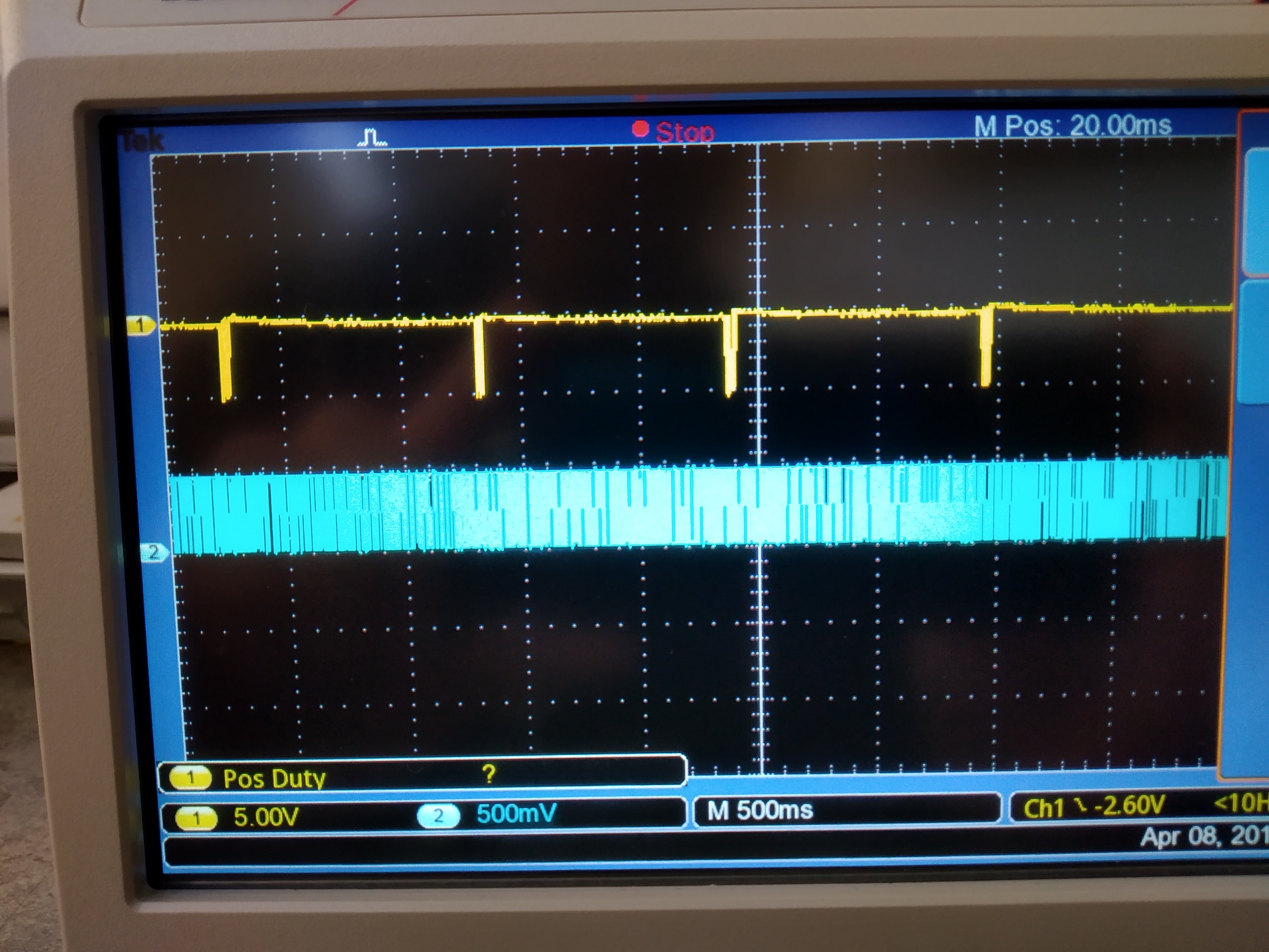
The following program uses bit banging again to generate a PWM signal, but this time the duty cycle is modulated sinusoidally. The PWM frequency is also considerably higher (approximately 100 Hz), so although the LED really is switching on and off, the human eye can’t see it happening. Instead, the LED appears to be continuously on, but with a brightness that varies with the duty cycle.

Run the program to verify that the LED pulsates sinusoidally, then read over the code carefully to confirm that you understand what each line is doing.

//
// Bit banging PWM with sinusoidal modulation
// Written by Ted Burke - 20-Apr-2021
//

void setup()
{
  pinMode(3, OUTPUT);
}

void loop()
{
  // PWM counter, period and duty cycle
  int counter, top = 100, dutycycle;

  // Sinusoidal modulation of duty cycle
  dutycycle = 50 + 45 * sin(millis()/1000.0);
  
  // Use a for loop to count from 0 up to 100
  for(counter = 0 ; counter < top ; ++counter)
  {
    digitalWrite(3, counter < dutycycle); // Set D3 high or low    
    delayMicroseconds(100); // Sets PWM frequency to approximately 100 Hz
  }
}

Once you’re sure you understand how the above program works, save a new copy of it called “sineLEDs” then try modifying it so that it modulates two LEDs out of phase with each other, as shown the following short video.

There are several ways you could approach this problem, but here are some suggestions:

Add a second LED and 220Ω resistor to the circuit.
In the program, create an additional digital output pin.
Look at the lines in the original program that switch the first LED on and off. You’ll need to add something similar to control the second LED in the opposite way.

SUBMISSION ITEM 2: Record a 20-second video of your two LEDs pulsating out of phase with each other. Name the file “sineLEDs.mp4” (or .avi or .mkv or whatever). Submit your video file to Brightspace.

Part 3: PWM output using the Arduino library’s analogWrite function

The primary disadvantage of bit banging is that it uses up processor time and makes it difficult to get anything else done because the microprocessor is so busy switching the pin high and low all the time. Fortunately, like many other microcontrollers, the ATmega328P (the brain of the Arduino Nano) has several hardware modules that can generate PWM signals in the background while the microprocessor gets on with other tasks.

The easiest way to output PWM signals from an Arduino Nano is using the “analogWrite()” function which is provided by the Arduino libraries, but it imposes certain limitations: Only some of the pins can be used and for each pin, the PWM frequency is fixed. Specifically,

Pins D3, D9, D10 and D11 can output 490 Hz PWM.
Pins D5 and D6 can output 980 Hz PWM.

Note that the specific pins and PWM frequencies vary from one model of Arduino to another. Also, it’s worth noting that by programming the low level registers that configure the ATmega328P’s hardware PWM modules, the frequency can be set to different values. However, this is beyond the scope of today’s lab. More details can be found in chapters 14-17 of the ATmega328P datasheet.

To understand how the analogWrite function works, read the official documentation page on the Arduino website. Using the same circuit as in the previous part, try running the example program below. Having read the analogWrite documentation, hopefully the program will be self-explanatory.

void setup()
{
  pinMode(3, OUTPUT);
}

void loop()
{
  // Increase LED brightness in steps
  analogWrite(3, 0);   // 0% duty cycle
  delay(1000);
  analogWrite(3, 16);  // 6.25% duty cycle
  delay(1000);
  analogWrite(3, 32);  // 12.5% duty cycle
  delay(1000);
  analogWrite(3, 64);  // 25% duty cycle
  delay(1000);
  analogWrite(3, 128); // 50% duty cycle
  delay(1000);
  analogWrite(3, 255); // 100% duty cycle
  delay(1000);
}

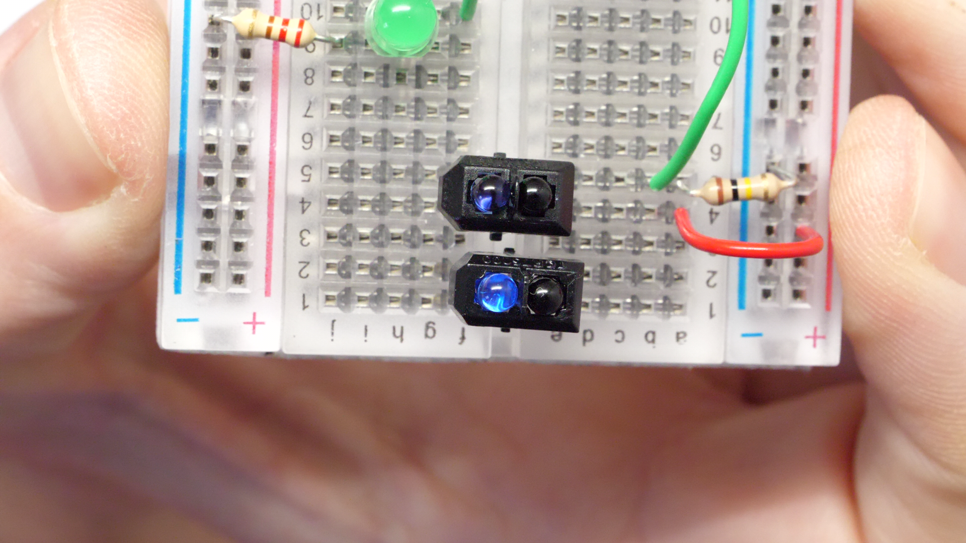
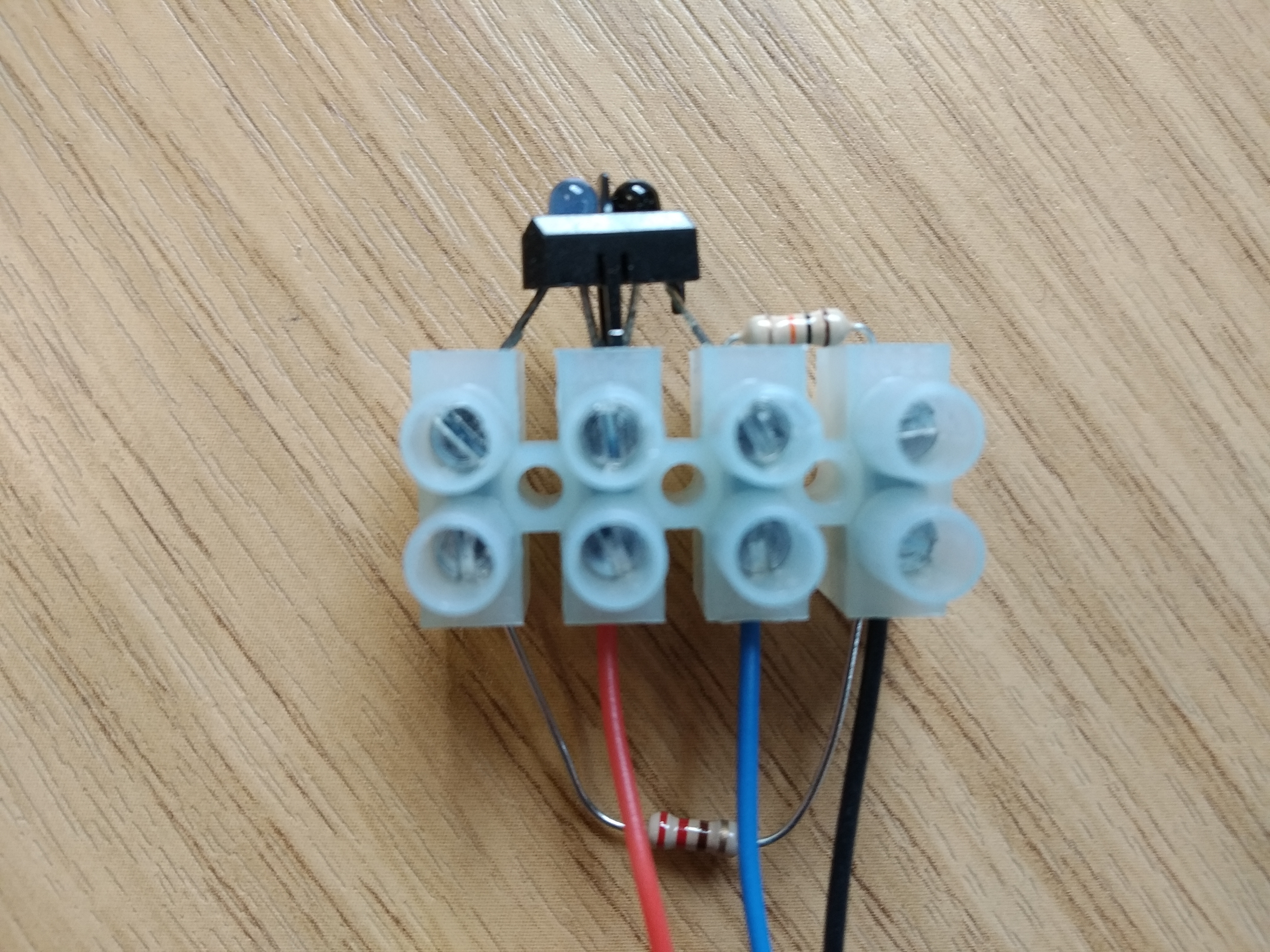
Using the Arduino’s analogRead and analogWrite functions, write a program that allows a TCRT5000 sensor to control the brightness of an LED, as shown in the following short video. As explained in the Arduino documentation (and as you have seen before), the analogRead function returns a value between 0 and 1023, whereas the analogWrite function accepts duty cycle values between 0 and 255. Hence, you will probably need to divide down each value you read from the analog input before using it to set the PWM duty cycle.

SUBMISSION ITEM 3: Record a 10-second video of your LED brightness responding to the TCRT5000 sensor. Name the file “TCRT_LED.mp4” (or .avi or .mkv or whatever). Submit your video file to Brightspace.

Part 4: Motor speed control using PWM

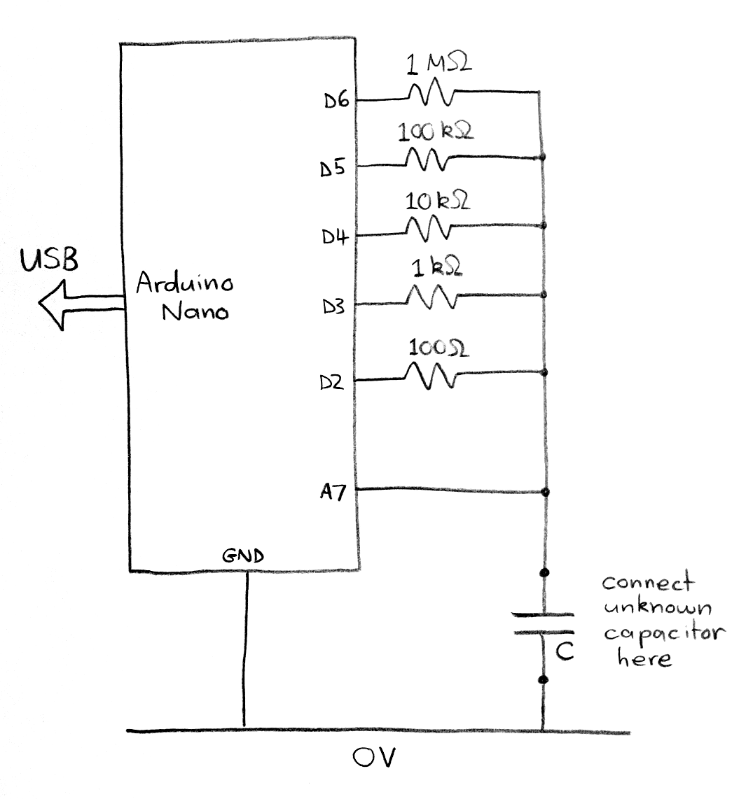
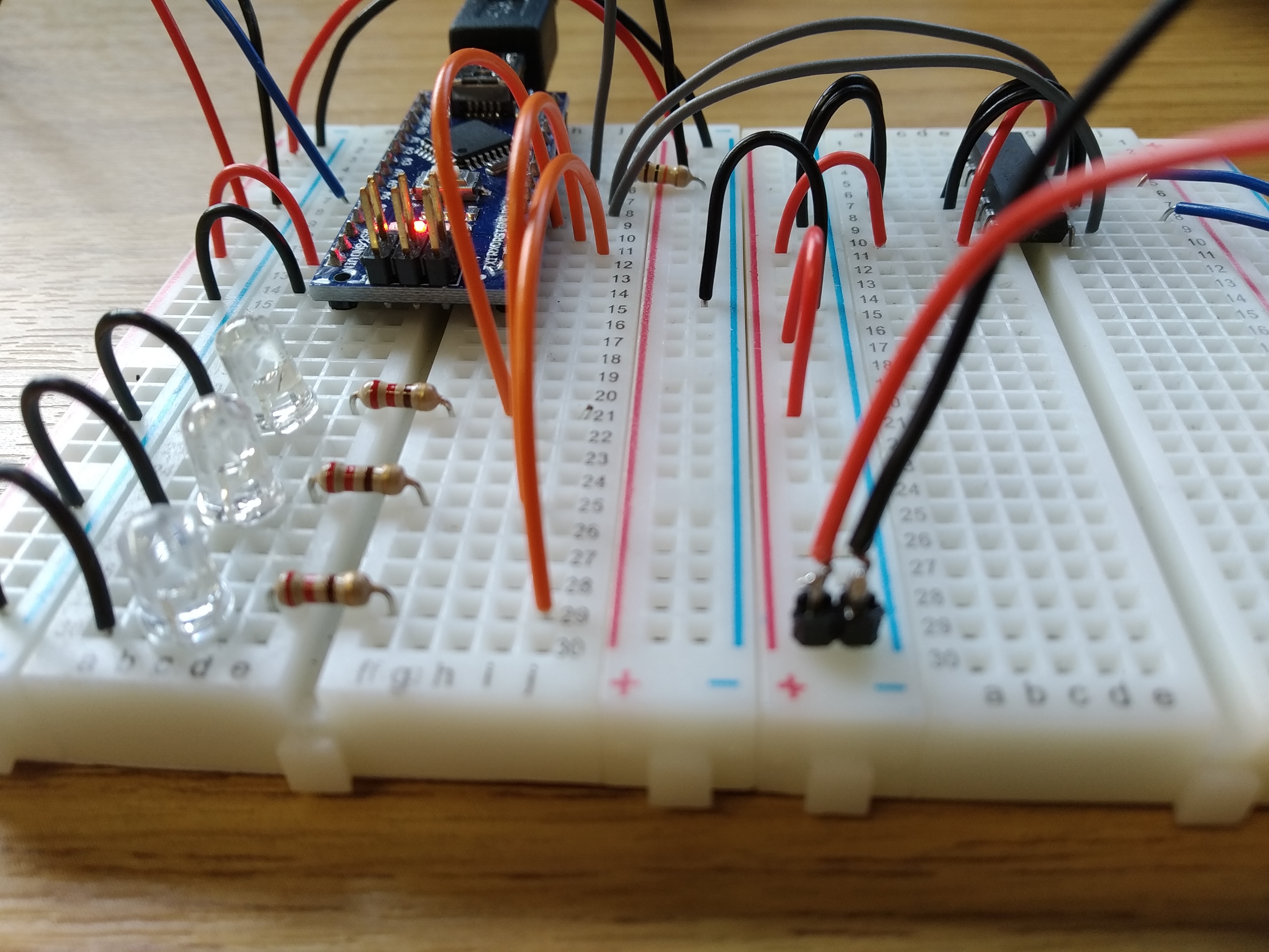
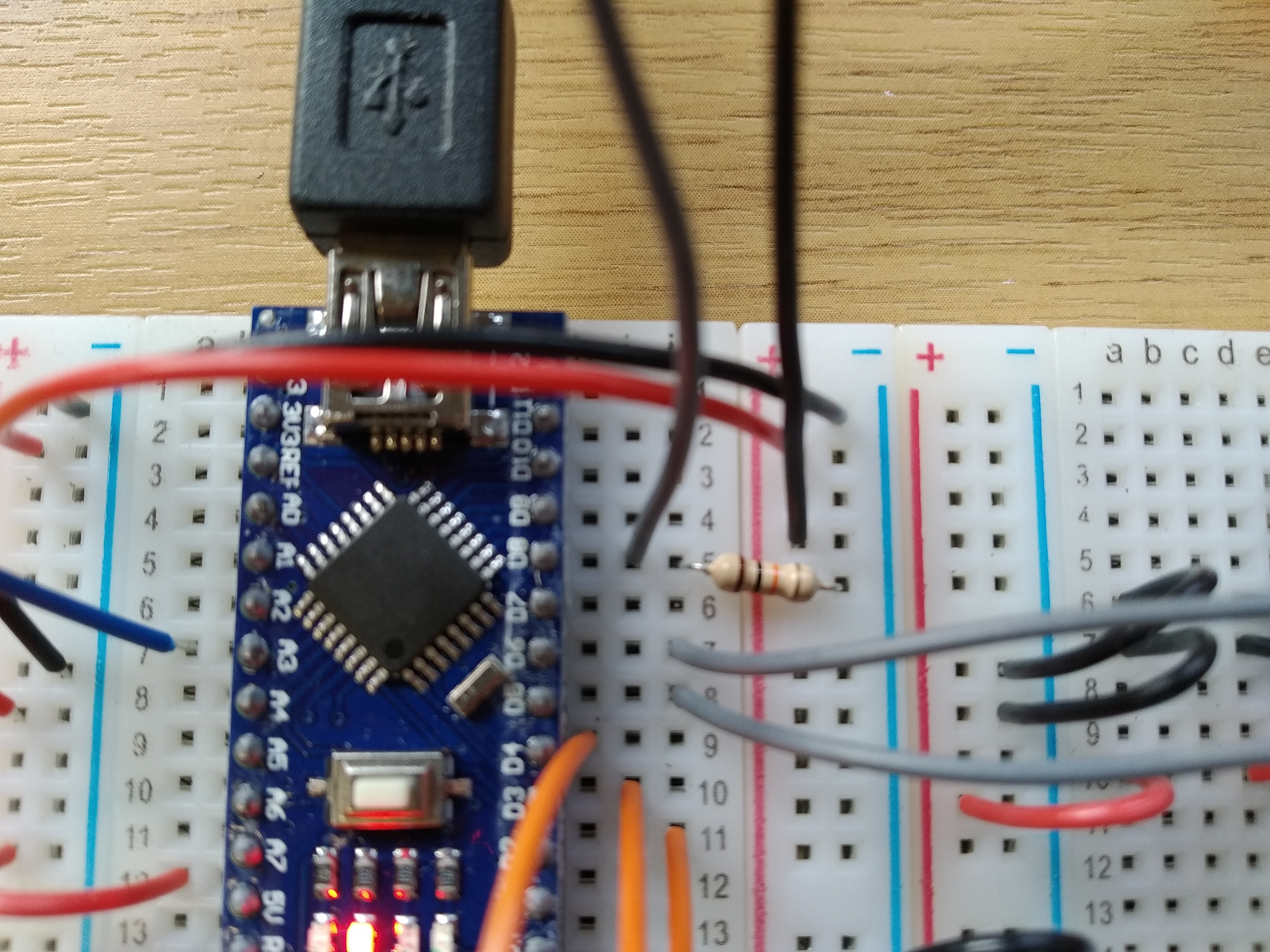
In this part, we will use PWM to control the speed of a motor. Construct the following circuit:

As explained in the SN754410NE datasheet, pins 1 and 9 on that chip are “enable” pins. When the voltage on pin 1 is high, the two outputs on that side of the chip (pins 3 and 6) are enabled; when the voltage on pin 1 is low, pins 3 and 6 are disabled. By injecting a PWM signal into pin 1, the power supplied to the motor becomes intermittent rather than constant. In essence, the duty cycle of the PWM signal controls the amount of power delivered to the motor and hence its speed.

Try running the following (hopefully self-explanatory) program and verify that the motor moves as expected.

void setup()
{
  pinMode(3, OUTPUT); // PWM output pin
  
  pinMode(4, OUTPUT); // motor forward
  pinMode(5, OUTPUT); // motor reverse
}

void loop()
{
  // Motor forward at 50% for 2 seconds
  digitalWrite(4, HIGH);
  digitalWrite(5, LOW);
  analogWrite(3, 128); // 50% duty cycle
  delay(2000);
  
  // Motor forward at 100% for 2 seconds
  digitalWrite(4, HIGH);
  digitalWrite(5, LOW);
  analogWrite(3, 255); // 100% duty cycle
  delay(2000);
  
  // Motor reverse at 50% for 4 seconds
  digitalWrite(4, LOW);
  digitalWrite(5, HIGH);
  analogWrite(3, 128); // 50% duty cycle
  delay(4000);
}

Modify the program to perform the following sequence repeatedly:

Forward for 2 seconds at 50% duty cycle,
Stop for 2 seconds,
Reverse for 1 second at 100% duty cycle,
Stop for 2 seconds.

SUBMISSION ITEM 4: Record a 20-second video of your motor performing the above sequence. Name the file “motor.mp4” (or .avi or .mkv or whatever). Submit your video file to Brightspace.

Part 5: Remote control of motor speed

Previously, we used the Serial Monitor to display text printed from the Arduino on the screen of the PC. In this final part of today’s lab, we will use the Serial Monitor tool in a new way – to send commands from the PC to the Arduino. This will allow the motor speed and direction to be controlled remotely.

Using the same circuit as in the previous part, run the following program.

//
// Motor speed remote control example
// Written by Ted Burke - 20-Apr-2021
//

void setup()
{
  Serial.begin(115200);

  pinMode(3, OUTPUT); // PWM output for motor speed control
  
  pinMode(4, OUTPUT); // motor forward
  pinMode(5, OUTPUT); // motor reverse
}

void loop()
{
  int command_char; // incoming command character
  int motor_speed;

  // Check if any characters have been received
  if (Serial.available() > 0)
  {
    // Read the command character
    command_char = Serial.read();

    // Process the forward command if necessary
    if (command_char == 'f')
    {
      motor_speed = Serial.parseInt();
      
      Serial.print("forward ");
      Serial.println(motor_speed);
      
      analogWrite(3, motor_speed);
      digitalWrite(4, HIGH); // forward
      digitalWrite(5, LOW);      
    }

    // Process the stop command if necessary
    if (command_char == 's')
    {
      Serial.println("stop");
      
      digitalWrite(4, LOW); // stop
      digitalWrite(5, LOW);      
    }
  }
}

At the top of the Serial Monitor window, there is a text box for sending messages to the Arduino. The motor can be controlled by typing commands into this text box and pressing enter (or clicking the “Send” button). The program above responds to two commands: “f” for forward and “s” for stop. The forward command should include an integer value between 0 and 255 for the motor speed. For example, to set the motor driving forward at 50% duty cycle, type “f128”. The stop command is just the single character “s” and does not require a numerical value. Try the program out for yourself and verify that you can control the motor. Read the program carefully to figure out how it works. It includes two new functions from the Arduino library that we have not used before: Serial.available() and Serial.parseInt(). Read the documentation pages to learn about what each one does.

Your final task is to modify the previous program to add a third command: “r” for reverse. It should function the same as the forward command, except that the motor turns in the opposite direction.

SUBMISSION ITEM 5: Save your Arduino program as “motorCommands” and submit the file “motorCommands.ino” to Brightspace. Please ensure that your code is neatly indented and fully commented (including your name and date at the beginning).

2020-21 Sem 2 Lab 7: Binary Signal Detective

There are three parts to today’s lab. Each part deals with a different aspect of binary signal analysis.

Part 1: Decode a 4-letter word from a binary signal

The animated gif image below contains a binary signal, that has a short message encoded in it:

The message encoded in the signal is a 4-letter word. Using a phototransistor and an Arduino, the signal can be recorded and plotted on the screen so that the message can be decoded.

Each byte contains 8 data bits.
Each byte is preceded by a start bit (1).
Each byte is followed by a stop bit (0).
Bytes are transmitted least significant bit (lsb) first.
Each byte represents one text character using UTF-8 / ASCII encoding.

Each byte represents one character of text using UTF-8 / ASCII encoding. Tables of UTF-8 / ASCII character values are widely available online, such as this one on Wikipedia. The 4-letter key word encoded in the example signal shown above is “Demo”.

The list below includes an animated gif file for each student in the class. A unique 4-letter key word is encoded into each gif file. Your instructor will tell you which gif is assigned to you. Your goal is to use your Arduino (with a TCRT5000) to record and plot the binary signal encoded in your gif and then decode it to reveal your 4-letter key word. Once you find your keyword, submit it to the Brightspace assignment set up for today’s lab.

The circuit shown below can be used to convert the optical signal into a voltage signal and then record it using an Arduino.

The following Arduino program samples the analog voltage on pin A0 every 10 ms and prints the value (in digital units) via the serial connection. This allows the signal to be displayed on the screen using the Serial Monitor or Serial Plotter in the Arduino IDE.

//
// optoscope.ino - written by Ted Burke - 23 Mar 2021
// This program measures the analog voltage on pin A0
// every 10ms and prints the value in digital units.
//

void setup()
{
  // Open serial connection at 115200 baud
  Serial.begin(115200);
}

void loop()
{
  unsigned long t_next; // next sample time

  t_next = micros(); // initialise sample time

  while(1)
  {
    // Wait 10000us between samples
    t_next = t_next + 10000L;
    while(micros() < t_next);

    // Print a sample from pin A0
    Serial.println(analogRead(0));
  }
}

If the Serial Monitor is used, the signal appears as a list of numbers that can be copied and pasted into a CSV file, and then be loaded into Octave / MATLAB and plotted for detailed analysis. If the signal is contained in a CSV file called “data.csv” then the following Octave commands can be used to load and plot the data:

data = csvread('data.csv');
plot(data);

SUBMISSION ITEM 1: Submit your 4-letter key word to Brightspace.

If you have problems getting a signal from your screen in Part 1: Workaround for TCRT5000

It has emerged that some of the TCRT5000s in the student kits do not respond at all to the visible light emitted by computer/phone screens. If the signal measured by your circuit responds well when you hold a TV remote against it and press and button, or when you move your hand over it to block the daylight (which contains IR light), but it does not respond at all when you hold it up to the flashing gif on the screen, then your circuit is probably wired correctly, but you have one of these problematic TCRT5000 sensors. It’s worth nothing that this is not actually a fault with your TCRT5000 – we’re using this component to sense something it wasn’t designed to sense (visible light).

Anyway, the first possible workaround is to try a different TCRT5000, because some of the ones in the kits work perfectly as described in Part 1. The photo below shows two TCRT5000s, one which responds to light from the screen (the bottom one) and one which does not (the top one). As you can see, the one that responds to the screen has a paler “blue eye” (the LED).

The second workaround is to rewire your circuit as shown below, so that the LED is actually emitting IR light and the sensor detects how much of it is reflected from the screen. This is different from what was described in Part 1, because in that case the sensor was sensing light that was emitted from the screen rather than reflected off it.

Using this workaround, the signal will not appear as strong as it would using the original method described in Part 1. With care though, it should be possible to obtain a clear signal. You may need to adjust the angle very carefully to get a good response. The TCRT5000 should be pressed right up against the screen. In this case, it actually seems to work better if you hold it at a slight angle (20 or 30 degrees) rather than pointing straight into the screen. The flashing gif below can be used for testing, together with the Serial Plotter in the Arduino IDE. The waveform below shows what kind of response you can hope to see when you have the sensor positioned correctly.

Part 2: Record a binary signal from an infrared remote control

Most TV remote controls use pulses of infrared light to transmit information to the appliances they control. These infrared pulses form a binary signal and each button produces a different series of ones and zeros. Different manufacturers use different communication protocols.

Try to capture a clear plot of the binary signal produced by your remote control. The figure below shows an example binary signal captured from a Panasonic TV remote control. Each of the pulses visible below actually consists of a short burst of some carrier frequency (normally around 38 kHz). Hence, if you zoom in very close, you may notice that the pulses aren’t completely solid.

The binary signals produced by a remote control are a lot faster than the (very slow) signal you decoded in Part 1. To capture the fast-changing detail in the remote control signal, some changes to the Arduino circuit are required, as shown below. The resistor value is reduced to 1 kΩ and the signal is sampled through a digital input pin rather than an analog input.

The Arduino program shown below waits until a rising edge is detected on digital input pin D3. As soon as a rising edge is detected, the Arduino captures 10000 samples of the binary signal at a sampling rate of 100 kHz. The samples are stored to a memory buffer during recording, then printed out via the serial connection once recording is complete. (EDIT 13-Apr-2021: Added a line to reset the data buffer to all zeros before capturing each transmission, which ensures that none of the previous transmission’s samples remain in the buffer.)

//
// Remote control binary signal capture example code
// Written by Ted Burke - last updated 13-Apr-2021
//
 
unsigned char data[1250];  // 1250-byte buffer to store 10000 bits
unsigned int n = 0;        // sample counter

void setup()
{
  Serial.begin(115200);    // open serial connection
}
 
void loop()
{
  for(n=0 ; n<1250 ; ++n) data[n] = 0; // reset data buffer to all zeros
  
  while(!digitalRead(3));  // wait for start of transmission

  // Record 10000 samples into the data buffer
  for(n=0 ; n<10000 ; ++n)
  {
    // Record a 1-bit sample from pin D3 into the buffer
    // Eight samples get packed into each byte in the buffer
    data[n/8] += digitalRead(3) << (n%8);
 
    // Precise delay to get very close to 100 kHz sampling
    delayMicroseconds(3);
    __asm__("nop\n\tnop\n\t"); // tiny delay!
  }
 
  // Print out the stored samples
  for(n=0 ; n<10000 ; ++n) Serial.println((data[n/8] >> (n%8)) & 1);

  delay(500);
}

The signal can be copied and pasted from the Serial Monitor into a CSV file and then loaded into Octave/MATLAB for plotting and analysis (see example Octave commands in Part 1).

Try plotting the signals for different buttons on your remote control. Can you see how the signal changes for different buttons?
Search online for information about the communication protocol used by your remote control. Can you find a matching protocol online?
How are ones and zeros represented in the signal emitted by your remote control?

SUBMISSION ITEM 2: If you captured clear signals from your remote control, then paste some example plots into a Word document and submit it to the Brightspace assignment. If you tracked down any information online about the protocol used by your remote control, include that information in the Word document (a summary and/or links to the information online).

Part 3 (advanced): Program the Arduino to respond to the remote control

Once you have established how your remote control encodes each of its buttons, try to write an Arduino program that prints two different messages (via the Serial Monitor) when two different buttons are pressed on the remote control.

Note that this is much more difficult than the tasks in Parts 1 and 2. If you’re not sure where to start, discuss it with your lab instructor. The solution will be different for each remote control, because it will depend on the signal encoding used. Here are some ideas to get you started:

A good place to start is to get the Arduino to respond to any button.
If you only need to tell the difference between two buttons, then look for any single point that’s different in the two signals and focus on that. Measure the time delay from the start of the message to that point in the signal. If you check the signal level at that exact time, you should be able to determine which of the two signals it is.
Try discussing the problem with you classmates and your lab instructors.

SUBMISSION ITEM 3: If you get this part working, record a short video showing the Arduino responding to each button and submit it via Brightspace. Please upload your “.ino” file also.

Appendix: Some useful / interesting information

Notes from yesterday’s lecture:

In case you’re curious how those binary signal gifs were generated…

The following C program creates two PGM images, “0.pgm” and “1.pgm”, that are used as frames in the generated gif animations. Each image is 100 x 100 px. “0.pgm” is all white. “1.pgm” is all black.

//
// make_bw_frames.c - written by Ted Burke - 22 Mar 2021
// Make black and white frames for creating binary signal gifs
//
// To convert frames to gif using ImageMagick:
//      
//      convert -delay 25 -loop 0 *.pgm flash.gif
//

#include <stdio.h>

// Image height and width in pixels
#define H 100
#define W 100

void print_pgm(FILE *f, int h, int w, int n);

int main()
{
    FILE *f;
    
    // Write a white square to a PGM file
    f = fopen("0.pgm", "w");
    print_pgm(f, H, W, 255);
    fclose(f);
    
    // Write a black square to a PGM file
    f = fopen("1.pgm", "w");
    print_pgm(f, H, W, 0);
    fclose(f);  
}

void print_pgm(FILE *f, int h, int w, int n)
{
    int x, y;
    
    // Print the contents of a PGM file containing
    // a solid rectangle of the specified width,
    // height and pixel value
    fprintf(f, "P2\n%d %d\n255\n", w, h);
    for (y=0 ; y<h ; ++y)
    {
        for (x=0 ; x<w ; ++x)
        {
            // Print pixel value
            fprintf(f, "%03d ", n);
        }
        fprintf(f, "\n");
    }
}

A file similar to the one shown below called “keys_list.txt” must then be provided. A gif file will be created for each line.

01	Blip
02	dark
03	SHOE
04	Harp
...

The following program reads the keys and numbers from “keys_list.txt” and generates an animated gif file for each line. It uses ImageMagick’s convert utility to create each gif. Two frame images – “0.pgm” and “1.pgm” – must be present in the same folder – one being a plain black image and the other being a plain white image.

//
// make_gifs.c - written by Ted Burke - 23 Mar 2021
//
//    gcc make_gifs.c -o make_gifs
//

#include <stdio.h>
#include <string.h>
#include <stdlib.h>

int main()
{
    int i, j, n, number;
    char key[10];
    
    // Buffer to store ImageMagick command for creating each gif
    char command[2000];
    
    FILE *f = fopen("keys_list.txt", "r");
    
    for (n=1 ; n<=26 ; ++n) // create 26 gif files
    {
        // Read gif number and key word from keys_list.txt
        fscanf(f, "%d %s", &number, key);
        
        // Construct ImageMagick command to create gif animation
        sprintf(command, "convert -delay 25 -loop 0 ");
        
        // Add one frame to animation for each bit (40 frames in total)
        for (i=0 ; i<4 ; ++i) // 4 bytes
        {
            sprintf(command + strlen(command), "1.pgm ");  // start bit
            for (j=0 ; j<8 ; ++j) // 8 bits in each byte
            {
                // next data bit
                if ((key[i] >> j) & 1) sprintf(command + strlen(command), "1.pgm ");
                else sprintf(command + strlen(command), "0.pgm ");
            }
            sprintf(command + strlen(command), "0.pgm "); // stop bit
        }
        
        // Leave a long gap (40 frames) before next transmission
        for (i=0 ; i<40 ; ++i) sprintf(command + strlen(command), "0.pgm ");
        
        // Complete the ImageMagick command by adding output filename
        sprintf(command + strlen(command), "%02d.gif\n", number);
        
        //printf("\n%s\n", command);
        
        // Execute ImageMagick command to create gif
        system(command);
    }
    
    fclose(f);
    
    return 0;
}

The following Arduino program was used to measure the sampling rate when recording the remote control signal.

//
// Remote control binary signal capture example code
// Written by Ted Burke - 23-Mar-2021
//

const unsigned int N=10000;
unsigned char data[1250];  // 1250-byte buffer to store 10000 bits
unsigned int n = 0;        // sample counter

void setup()
{
  Serial.begin(115200);    // open serial connection
}

void loop()
{
  unsigned long t1, t2, t; // used to calculate elapsed time
  
  while(!digitalRead(3));  // wait for start of transmission
  t1 = micros();           // remember time before sampling

  // Record 10000 samples into the data buffer
  for(n=0 ; n<N ; ++n)
  {
    // Record a sample from pin D3 into the buffer
    data[n/8] += digitalRead(3) << n%8;

    // Precise delay to get very close to 100 kHz sampling
    delayMicroseconds(3);
    __asm__("nop\n\tnop\n\tnop\n\tnop\n\t");
  }

  t2 = micros();
  t = t2 - t1;
  //Serial.print(t); Serial.println(" us");
  //Serial.print(N/(t*1e-6), 5); Serial.println(" Hz");
  //Serial.print(t/(float)N); Serial.println(" us/sample");

  // Print out stored samples
  if (1) for(n=0 ; n<N ; ++n) Serial.println((data[n/8] >> (n%8)) & 1);
}

2020-21 Sem 2 Lab 6: Simulation of series and parallel resonant RLC circuits

In this lab, you will work in teams to simulate two well-known circuits in LTspice. In each case, your objective is to replicate a provided screenshot, including a plot showing the result of a circuit simulation. To make the task more difficult, the value of a capacitor has been concealed in each screenshot. You may find it useful to do some impedance calculations in Octave / MATLAB to identify the correct capacitance value for each circuit.

As discussed in previous lectures, each of the three fundamental linear circuit elements can be converted to an impedance:

$Z_R = R \quad\quad Z_L = j \omega L \quad\quad Z_C = \frac{1}{j \omega C}$

where

Z_R is the impedance of a resistor [Ω]
R is resistance [Ω]
Z_L is the impedance of an inductor [Ω]
L is inductance [H]
Z_C is the impedance of a capacitor [Ω]
C is capacitance [F]
ω is angular frequency [rad/s]
j is the imaginary unit – i.e. $j=\sqrt{-1}$

Impedances in series

Two or more impedances in series can be combined into a single equivalent impedance, Z_eq, simply by adding them up:

$Z_{eq} = Z_1 + Z_2 + Z_3$

Impedances in parallel

Two impedances in parallel, Z₁ and Z₂, can be combined into a single equivalent impedance, Z_eq, as follows.

$\frac{1}{Z_{eq}} = \frac{1}{Z_1} +\frac{1}{Z_2}$

or equivalently

$Z_{eq} = \frac{Z_1 Z_2}{Z_1 + Z_2}$

Part 1: Series resonant RLC circuit

This circuit includes an inductance and capacitance in series, which causes it to resonate at one particular frequency (100 Hz in this case). The reactance of an inductor is positive, but the reactance of capacitor is negative. Both reactance values depend on frequency. When the frequency is just right, the two reactances cancel each other out perfectly, leaving only the small resistance to limit the current in the circuit. This is called the resonant frequency of the circuit.

The impedance of a series resonant RLC circuit is minimised at its resonant frequency.

Working with your teammates, replicate the screenshot shown above as precisely as you can. Please note the following:

The simulation type is set to “AC Analysis”. This produces a plot with frequency on the horizontal axis, showing how the circuit responds over a range of frequencies.
The label showing the capacitor value has been erased from the screenshot above, but it should be visible in your screenshot. You will have to figure out the value of the capacitor, for example by doing impedance calculations in Octave / MATLAB.
Set the background colour of the circuit diagram to white.
Add your name and the names of your teammates to the schematic (in place of the example names shown above).

SUBMISSION ITEM 1: Submit your LTspice screenshot of the series resonant circuit to Brightspace. Ensure your screenshot is as close as possible to the original example screenshot. Ensure that it includes your names. Although you are working in teams, each individual student should submit their own screenshot to Brightspace.

Part 2: Parallel resonant RLC circuit

This circuit features an inductor and a capacitor in parallel. Any actual physical inductor has some non-zero resistance, so a small resistance is included here in series with the inductor. Like the previous circuit, this one resonates at one particular frequency (1.8766 kHz in this case) and its impedance is purely real at that frequency (i.e. no imaginary part / zero reactance). However, unlike the series resonant circuit, the impedance of a parallel resonant RLC circuit is maximised at its resonant frequency.

Working with your teammates, replicate the screenshot shown above as precisely as you can. Please note the following:

The label showing the capacitor value has been erased from the screenshot above, but it should be visible in your screenshot. Try to calculate the value of the capacitor, for example using Octave / MATLAB.
Set the background colour of the circuit schematic to white.
Add your name and the names of your teammates to the schematic.

SUBMISSION ITEM 2: Submit your LTspice screenshot of the parallel resonant circuit to Brightspace. Ensure your screenshot is as close as possible to the original example screenshot. Ensure that it includes your names. Although you are working in teams, each individual student should submit their own screenshot to Brightspace.

Part 3: Extra circuit analysis exercise

If you finish parts 1 and 2 before the end of class, have a go at this additional circuit analysis problem. C_pfc is a power factor correction capacitor – do not include it for the initial calculation, but once you have calculated I_s and the total equivalent impedance, calculate the required value of C_pfc to bring I_s perfectly into phase with V_s.

2020-21 Sem 2 Lab 5: Computer simulation and analysis of AC circuits

In this experiment, you will investigate a series of AC circuits using two different approaches:

Phasor analysis using Octave / MATLAB,
Circuit simulation in LTspice.

You’ll install LTspice and Octave, then use them both to analyse each circuit.

There are seven submission items in total, each of which should be uploaded to the Brightspace assignment for today’s lab. Each item is either a screenshot or an m-file (a MATLAB/Octave program).

Install LTspice and Octave

LTspice is free circuit simulation software distributed by the semiconductor company Analog Devices. It’s one of a number of circuit simulation tools based on the open source circuit simulator SPICE, which was first released almost 50 years ago. LTspice can be downloaded here:

https://www.analog.com/en/design-center/design-tools-and-calculators/ltspice-simulator.html#

Scroll down to the “Download LTspice” section and click on “Download for Windows 7, 8 and 10“. Run the downloaded file to install LTspice on your machine.

MATLAB is a programming and numerical computing environment that is widely used by engineers to process and analyse signals and data. MATLAB is proprietary software, and purchasing a full license is very expensive. However, it’s an extremely powerful tool and many engineers spend a large part of their professional life working in it, so companies are willing to pay to use it. As a TU Dublin student, you can access MATLAB for free, but there are also a number of free software alternatives. GNU Octave is one of these. Octave is free and easy to install and the syntax is almost entirely identical to MATLAB. For today’s lab, everything you need to do will work perfectly in Octave, so we are suggesting that you download and install it from the following location:

https://www.gnu.org/software/octave/download

Scroll down to the “Microsoft Windows” section and download the first file, “octave-6.2.0-w64-installer.exe” which will install Octave on your machine.

If you can’t install Octave for some reason, these are other options you could consider:

Use Octave Online (somewhat limited, but would be fine for today’s lab),
Use MATLAB Online,
Download and install MATLAB.

Whichever option you use, the steps to carry out the circuit analysis will be essentially the same.

Part 1: Calculate the current in an RL circuit

The following video demonstrates the process of using MATLAB / Octave to calculate the current in an RL circuit and then using LTspice to simulate the circuit. Although the circuit shown in the video is very similar to the one you’ll be analysing here, please note that the component values are intentionally not the same.

Apply the same type of analysis to the following circuit using Octave and LTspice.

SUBMISSION ITEM 1: Submit your m-file. Ensure the file is neat and well commented. The first comment should provide your name, the date, and briefly explain the purpose of the program.

SUBMISSION ITEM 2: Submit an LTspice screenshot showing the circuit diagram and two full cycles of the waveforms v_s(t) and i_s(t). Make sure the simulation agrees with the results of your MATLAB/Octave analysis.

Part 2: Calculate the current in an RC circuit

Apply the same type of analysis (using Octave and LTspice) to the circuit shown below. Remember that the impedance of a capacitor is given by the following formula:

$Z_c = \frac{1}{j \omega C}$

SUBMISSION ITEM 3: Submit your m-file. Ensure the file is neat and well commented. The first comment should provide your name, the date, and briefly explain the purpose of the program.

SUBMISSION ITEM 4: Submit an LTspice screenshot showing the circuit diagram and two full cycles of the waveforms v_s(t) and i_s(t). Make sure the simulation agrees with the results of your MATLAB/Octave analysis.

Part 3: Series resonant circuit

The impedance of the RLC circuit shown below reaches a minimum value at its so-called resonance frequency, ω₀ [rad/s]. The current will therefore be at its maximum amplitude when

$f = \frac{\omega_o}{2\pi}$

Write an m-file to calculate the magnitude of the current for a given frequency, f [Hz]. By running the m-file repeatedly with a different value of f each time, create a graph of current magnitude versus frequency over the range $0 \leq f \leq 300 \:\mbox{Hz}$ .

SUBMISSION ITEM 5: Submit your m-file. Ensure the file is neat and well commented. The first comment should provide your name, the date, and briefly explain the purpose of the program.

SUBMISSION ITEM 6: Submit a screenshot of your graph. As always, include a title, axis labels, and units for each axis.

Part 4: Power factor correction

In the circuit below, a capacitor is placed in parallel with an RL load. The resistance and inductance values are specified but the capacitance is not. With the correct capacitance value, the current phasor I_s will be perfectly in phase with the supply voltage phasor V_s, which is is highly desirable because it’s more efficient to transmit electricity over long distances when the voltage and current are in phase. Hence, electricity providers provide substantial price incentives for large-scale commercial customers to keep their current in phase with the supply voltage, which (assuming an inductive load) can be achieved by installing capacitance to perform power factor correction (PFC). We will learn more about PFC in the coming weeks, but for now…

Can you figure out what value of C to include in the circuit to bring I_s into phase with V_s?

Simulate the circuit in LTspice and, if you can find the correct value for C, take a screenshot showing the circuit diagram and the voltage and current waveforms in phase with each other.

SUBMISSION ITEM 7: Submit your LTspice screenshot.

2020-21 Sem 2 Lab 4: Building a capacitor

The objective of this experiment is to construct a parallel plate capacitor from materials readily available in your home or in a grocery shop. Suggested materials include aluminium foil (for the conducting plates) and cling film (for the dielectric that separates the plates). You’re free to improvise with other materials, but please observe the following rules:

Comply with all government guidelines related to Covid-19.
Use only dry materials in your capacitor. No liquids!
Carefully assess any potential risks associated with the materials you’re using and avoid doing anything that might cause injury (e.g. cutting up aluminium cans which produces dangerously sharp edges).

You’re encouraged to try to make the capacitance large. However, we’re also interested in how densely you can cram the capacitance into a compact space. We’re hoping that some of you will impress us with creative solutions.

To give you time to develop something impressive, we’ll spend two weeks on this experiment. At the end, you’ll submit a written lab report on your work. An example report (for a different, but related experiment) will be provided to guide you in writing your own report.

Theory

The following equation gives the expected capacitance for an ideal parallel plate capacitor.

$C = \frac{\epsilon A}{d}$

where

C is the capacitance in farads [F],
$\epsilon$ is the absolute permittivity (often just referred to as the permittivity) of the dielectric (insulating material) that separates the conducting plates in farads per meter [Fm^-1],
A is the area of each plate in square metres [m²], and
d is the distance between the plates in metres [m].

Note that the dielectric thickness, d, shown in the above diagram is greatly exaggerated. In a real capacitor, the dielectric would typically be extremely thin in order to get the plates as close to each other as possible.

Permittivity is a property of a material or medium in which an electric field is present. Tables of permittivity values are available for different materials (e.g. air, water, concrete, soil, glass, etc.). Permittivity has a very significant effect on how electromagnetic waves propagate through a medium so, among other things, it can tell us useful information about how mobile phone or wi-fi signals will penetrate the walls of a building. The medium with the lowest possible permittivity is a perfect vacuum. The permittivity of other materials are often provided as relative permittivity – the ratio between their absolute permittivity and the absolute permittivity of a vacuum.

$\epsilon = \epsilon_r \epsilon_0$

where

$\epsilon$ is the absolute permittivity of the material in question in farads per metre [Fm^-1],
$\epsilon_r$ is the relative permittivity of the material, which is a dimensionless value (i.e. it has no units because it’s the ratio of two values that are in the same units), and
$\epsilon_0$ is the permittivity of a vacuum, 8.854188 ✕ 10^-12 farads per metre [Fm^-1].

The permittivity of air is very close to that of a vacuum, so it has a relative permittivity of approximately 1. Materials that are good insulators tend to have low relative permittivities. Have a look online for some of the published lists of material permittivities.

Part 1: Prepare the capacitance meter

You will use the capacitance meter you built last week to test your newly built capacitor. Please upload the code below to the Arduino. It includes some modifications that improve the accuracy of the meter when measuring large capacitances (up to 1000 μF). The capacitance you achieve in the capacitor you build is more likely to be in the nanofarad range, but there’s no harm updating the meter just in case you do achieve a larger capacitance than expected.

Once you’ve updated the code on the capacitance meter, check that it’s still functioning correctly by measuring the capacitance of one of the known capacitors in your kit (e.g. 100 μF).

//
// EEPP Arduino capacitance meter
// Written by Ted Burke - last updated 15-Feb-2021
//
// This system (hardware circuit and software) measures the time
// constant of an RC circuit in order to calculate the value of
// the capacitor. To obtain a time constant of appropriate length,
// the system has five resistor values (100, 1k, 10k, 100k, 1M).
// The 100 ohm resistance is only used for charging the capacitor.
// The other four resistances are tried one at a time until a time
// constant longer than 50ms is observed, at which point the
// capacitance is calculated and printed via the Serial Monitor.
//
 
void setup()
{
  pinMode(2, INPUT); // disable 100 ohm resistor
  pinMode(3, INPUT); // disable 1k resistor
  pinMode(4, INPUT); // disable 10k resistor
  pinMode(5, INPUT); // disable 100k resistor
  pinMode(6, INPUT); // disable 1M resistor
 
  Serial.begin(115200); // open serial connection
}
 
void loop()
{
  int n; // resistor/pin number, e.g. R3 is 10^3 ohms and on pin D3 
  float tau, R, C; // time constant, resistance, capacitance
   
  // Try the resistors in this order: 1k, 10k, 100k, 1M.
  // The resistance used is equal to 10^n, so the value of n is
  // incremented until a time constant over 50ms is observed.
  // That time constant is then used to calculate the capacitance.
  n = 3;
  while (1)
  {
    tau = measureTimeConstant(n);
    if (tau > 50e-3) break;
    if (n == 6) break;
    if (tau == 0) n = 3; // go back to lowest resistance (1k)
    else n++;            // move up to higher resistance
  }
 
  // Calculate the resistor and capacitor values
  R = pow(10,n);
  C = tau / R;
 
  // Display the time constant, resistance and capacitance
  Serial.print("tau="); Serial.print(1000*tau, 3); Serial.print(" ms, ");
  Serial.print("R="); Serial.print(R, 0); Serial.print(" ohm, ");
  Serial.print("C=");
  if      (C < 1e-9) {Serial.print(C*1e12, 3); Serial.print(" pF");}
  else if (C < 1e-6) {Serial.print(C*1e9 , 3); Serial.print(" nF");}
  else if (C < 1e-3) {Serial.print(C*1e6 , 3); Serial.print(" uF");}
  else               {Serial.print(C*1e3 , 3); Serial.print(" mF");}
  Serial.println();
}
 
// This function measures the time constant in seconds using resistor n.
float measureTimeConstant(int n)
{
  unsigned long t1, t2, timeout;
  float Vth;
   
  // Charge the capacitor up to its maximum through the 100 ohm resistor.
  pinMode(2, OUTPUT);
  digitalWrite(2, HIGH);
  delay(1000);
  pinMode(2, INPUT);
 
  // Calculate the threshold voltage as 36.8% of the initial voltage.
  // The capacitor voltage drops to this value after one time constant.
  Vth = 0.36788 * analogRead(7);
   
  // Measure the time constant
  t1 = micros();              // record the start time in microseconds
  timeout = t1 + 1200000L;    // set timeout limit at 1.2 seconds
  pinMode(n, OUTPUT);         // enable the selected resistor
  digitalWrite(n, LOW);       // begin discharging the capacitor
  while(analogRead(7) > Vth)  // wait until voltage drops to Vth (or timeout)
    if (micros() > timeout) return 0;
  t2 = micros();              // record the end time in microseconds
  pinMode(n, INPUT);          // disable the selected resistor
  return (t2 - t1) * 1e-6;    // return the time constant (t2 - t1)
}

The circuit is exactly the same as it was in part 4 of last week’s lab.

This is the circuit on the breadboard. The capacitor near the top left corner of the breadboard is just there as an example. Remove that capacitor before plugging in the wires of your newly built capacitor to measure its capacitance.

Part 2: Construct a simple parallel plate capacitor

To begin with, construct a simple capacitor as follows:

Cut out two square pieces of aluminium foil, approximately 20 cm x 20 cm, but leaving an extra strip of foil extending from one corner of each piece (for attaching wires).
Cut two long wires – long enough to reach from the breadboard to opposite corners of your 20 cm x 20 cm square capacitor. Remove the insulation from the last 2 cm of each wire.
Sellotape one wire onto the corner strip of each piece of foil.

Lay one piece of foil down smooth flat surface.
Lay a piece of A4 paper on top of the foil, taking care to cover every part of it except for the strip with the wire attached.
Lay the second piece of foil down so that it is directly above the first piece (but separated from it by the paper). Orient it so that the corner with the wire attached is not at the same corner as the wire for the lower plate.
Lay something flat and heavy (like a hardback book) on top to press the three layers tightly together.

Plug the wires of your capacitor into your breadboard to measure its capacitance. (To give you a rough idea what to expect, when I tried building this capacitor I obtained a capacitance of approximately 15 nF.)
Try pressing down hard on the stack to squeeze the plates ever closer together. Does it affect the measured capacitance?
Using the equation from the theory section above, estimate the expected capacitance of this capacitor and compare it to the measured value. When applying the formula, note the following:
- The area of the plates must be expressed in square metres.
- The distance between the plates should be approximately equal to the thickness of the paper sheet. This is difficult to measure directly, but if you measure the height of a stack of sheets then divide by the number of sheets, a reasonably accurate estimate can be obtained. This distance must be expressed in metres.
- Different types of paper will have different relative permittivities. The exact value for the paper you’re using won’t be possible to find, but you should be able to find a reasonable ballpark estimate online.

Retain all your calculations, measurements, and links to information sources so that you can include them all in your lab report next week.

Part 3: Design, build and test a larger capacitor

Now you’re ready to create your own capacitor design, hopefully with a capacitance much greater than that achieved using the simple design described above.

Strategies to consider:

Increase the area of the plates?
Try a thinner dielectric material?
Use a dielectric with a different permittivity?
Stack more plates together?
Roll your capacitor into tightly rolled cylinder?
Create more than one capacitor and combine them in parallel?

Research online to get some more ideas.

Part 4: Write a lab report about the capacitor you built

An example lab report is now available in the Content section of the EEPP2 Brightspace module. The example report is for a different, but closely related, experiment. When you’re ready to write your report, you can use the example report as a template for writing your own account on this experiment. In the meantime, please retain or collect all of the following items:

Photographs of everything you built, ideally including steps during the build process.
Screenshots of anything you measured using the capacitance meter (i.e. the Serial Monitor window displaying the measurement).
Any calculations you carried out. If the calculations were carried out on paper, then retain the written calculations. If the calculations were carried out in MATLAB / Octave, then grab a screenshot or save it to an M-file so that you can refer back to it.
The sources of any information you obtained online – e.g. material permittivity, thickness of paper / cling film, etc.

2020-21 Sem 2 Lab 3: Building a capacitance meter

Theory

In this lab, we use what we have learned about the time constant of an RC circuit to build a capacitance measurement system. The basic principle is to construct an RC circuit using a known resistance and an unknown capacitance and then measure its time constant. The time constant, $\tau$ , of an RC circuit is given by the following equation.

$\tau = RC$

Hence,

$C = \frac{\tau}{R}$

In each part of this experiment, we measure the time constant by charging the capacitor to a maximum voltage and then allowing it to discharge through a resistor. The time it takes for the capacitor voltage to drop to 36.8% of its initial value is measured – this is the time constant.

For example, the diagram below illustrates what happens when a voltage source connected to an RC circuit suddenly drops from its initial value down to zero (at time t₁). Assuming the voltage source had been at its initial voltage long enough for the system to settle, then the capacitor is fully charged until time t₁ when it begins to discharge. The time constant provides a simple description of how fast the voltage drops towards its new resting level (0 V in this case).

In the first part of the lab, you will use the ASGO to capture a step response (of a negative-going step) and then analyse the data in Excel to find the time constant and calculate the capacitance. In parts 3 and 4, you will program the Arduino to measure the time constant automatically and print out the estimated capacitance.

In next week’s lab, you will construct your own capacitor from scratch using aluminium foil and other materials. The meter you build this week will allow you to measure the capacitance of your homemade capacitor next week.

Part 1: Measure capacitance by analysing a step response

In this part of the experiment, you will use the ASGO to capture the step response of an RC circuit and then analyse it in Excel to measure the time constant and hence obtain the capacitance. Construct the circuit shown below, using the ceramic (yellow) capacitor that is marked with the text “105M” (I won’t tell you the capacitance value, but the measurement you’re about to do should tell you what it is!).

Please note that I have rotated the MCP4911 DAC chip by 180 degrees since last week’s experiment – i.e. pin 1 of the DAC. is now in row 9 of the breadboard. You don’t need to rotate yours – I just thought it would be neater this way.

Upload the following code to the Arduino to generate a negative-going step voltage and record the response of the RC circuit.

//
// ASGO - Arduino Signal Generator and Oscilloscope
// Negative-going step response version
// Written by Ted Burke - last updated 9-Feb-2021
//
// Outputs a step waveform via a MCP4911 DAC IC, while
// simultaneously sampling the analog voltages on pins A0 and
// A1 and storing them to buffers. The input signal is generated
// for 1 second, of which the last 200 ms is recorded at a
// sampling frequency of 2 kHz. The step change occurs 20 ms
// after recording begins. 
//
// To generate a step and output a frame of sampled data to the
// Serial Monitor or Serial Plotter, set the baudrate to 115200
// and then send the text command "c" or "s" (for comma- or
// space-delimited data respectively).
//
  
#include <SPI.h>
#define SS_PIN 10
  
// Modify the following 2 lines to control the step input
const float v1 = 4.0;          // voltage before step [V]
const float v2 = 0.0;          // voltage after step [V]
 
// Convert initial and final step voltages to ints for writing to DAC
const int v1_int = 0.2 * 1023.0 * v1;
const int v2_int = 0.2 * 1023.0 * v2;
 
// Sampling frequency - do not change this!
const float fs = 2000;         // sampling frequency (input and output)
  
// Waveform buffers
int n = 0;                     // buffer index variable
const int N = 400;             // buffer length in samples
unsigned int buffer0[N] = {0}; // buffer for input A0
unsigned int buffer1[N] = {0}; // buffer for input A1
  
// Variables for interaction between main loop and Timer1 ISR
volatile int countdown1000ms = 0;
volatile int countdown820ms = 0;
  
void setup()
{
  pinMode(SS_PIN, OUTPUT);    // Ensure that SS is set to SPI master mode
  digitalWrite(SS_PIN, HIGH); // Unselect the device
  
  SPI.begin();
  SPI.setBitOrder(MSBFIRST);
  SPI.setDataMode(SPI_MODE0);
  SPI.setClockDivider(SPI_CLOCK_DIV2);
    
  Serial.begin(115200);     // open serial connection at 115200 bits/s
  
  // Initialize Timer1 
  noInterrupts();           // disable interrupts while configuring Timer 1
  TCCR1A = 0;
  TCCR1B = (1 << WGM12) | (1 << CS10); // CTC mode and clock prescaler set to 1
  TCNT1  = 0;               // reset Timer1 counter
  OCR1A = 8000;             // interrupt frequency is 16e6 / 8000 = 2000 Hz
  TIMSK1 |= (1 << OCIE1A);  // enable timer compare interrupt
  interrupts();             // re-enable interrupts
}
 
void loop()
{
  char c = 0;
  
  // Check for incoming text command character
  if (Serial.available() > 0) c = Serial.read();
  
  // Print either a space-delimited or comma-delimited data frame
  if (c == 's' || c == 'c')
  {
    // Set the initial voltage
    dac_output(v1_int);
     
    countdown820ms = 1640;  // count down to step time
    countdown1000ms = 2000; // count down one second of samples
    while(countdown1000ms); // let ISR handle the recording
  
    // Now stop recording and print buffers to PC
    for (int m=0 ; m<N ; ++m)
    {
      Serial.print(m / 2000.0, 4);
      Serial.print(c == 's' ? ' ' : ','); // either a comma or a space
      Serial.print((5.0 / 1023.0) * buffer0[(n+m)%N], 3);
      Serial.print(c == 's' ? ' ' : ',');
      Serial.println((5.0 / 1023.0) * buffer1[(n+m)%N], 3);
    }
    Serial.flush();
  }
}
  
//
// ** Timer1 interrupt service routine (ISR) **
// This runs once every sample period, updating the
// DAC output voltage and sampling the input voltage
// on pins A0 and A1 and storing them to buffers.
//
ISR(TIMER1_COMPA_vect)
{
  if (countdown1000ms)
  {
    // update DAC voltage to generate sinusoid
    dac_output(countdown820ms ? v1_int : v2_int);
  
    // store voltages from A0 and A1 to sample buffers
    n = (n+1)%N; // increment sample buffer index    
    buffer0[n] = analogRead(0);
    buffer1[n] = analogRead(1);
     
    if (countdown820ms) --countdown820ms; // count down to step
    --countdown1000ms; // count down to end of recording
  }
}
  
// Write a 10-bit value to the DAC to update its output voltage
void dac_output(unsigned short data)
{
  // Construct 16-bit value (command and data bits)
  data &= 0x3ff;          // truncate data value to 10 bits
  boolean channel = 0;    // always zero for MCP4911
  boolean bufferVref = 0; // Vref input buffering disabled
  boolean gain2x = 0;     // 2x gain disabled
  boolean shdn = 0;       // output shutdown disabled
  uint16_t out = (channel << 15) | (bufferVref << 14) |
                  ((!gain2x) << 13) | (!shdn << 12) | (data << 2);
  
  // Transmit the 16-bit value
  digitalWrite(SS_PIN, LOW);         // select DAC chip
  SPI.transfer((out & 0xff00) >> 8); // high byte
  SPI.transfer(out & 0xff);          // low byte
  digitalWrite(SS_PIN, HIGH);        // unselect DAC chip
}

To check that the program and circuit are working correctly, open the Serial Plotter. Make sure the baudrate is set to “115200 baud”. Send the text command “c” from the send box and you should see signals like the ones below appearing in the Serial Plotter.

Close the Serial Plotter and open the Serial Monitor instead. Send the text command “c” again to capture a frame of data in CSV format. You should see data similar to the following appearing.

Copy and paste all of the data from the Serial Monitor into an Excel document, as shown below. You’ll need to scan down through the rows of data to identify the values of t1 and t2. The second Excel screenshot below shows exactly how to find t1 and t2. Once you have found both values, calculate $\tau$ and C and show them both clearly on your spreadsheet. Create a neat graph with clear labels like that shown below.

How to find t1 and t2:

SUBMISSION ITEM 1: Submit (to Brightspace) a screenshot of your Excel spreadsheet showing your graph and calculated capacitance value. Also submit the Excel document itself.

Part 2: Response of RC circuit to square wave input voltage

Using the same circuit as in part 1, upload the following code to the Arduino. This version of the ASGO code outputs a square wave.

//
// ASGO - Arduino Signal Generator and Oscilloscope
// Square wave version
// Written by Ted Burke - last updated 9-Feb-2021
//
// Outputs a square wave via a MCP4911 DAC IC,
// while simultaneously sampling the analog voltages on
// pins A0 and A1 and storing them to buffers.
//
// To output a frame of sampled data to the Serial Monitor or
// Serial Plotter, set the baudrate to 115200 and then send the
// text command "c" or "s" (for comma- or space-delimited data
// respectively).
//
   
#include <SPI.h>
#define SS_PIN 10
   
// Modify the following 3 lines to control the output waveform
const float dc = 2.5;          // d.c. voltage offset [V]
const float aw = 1.0;          // waveform amplitude [V]
const float fw = 10;           // waveform frequency [Hz]
   
// Set sampling frequency - do not change this!
const float fs = 2000;         // sampling frequency (input and output)
const float inc = fw * 2.0 * M_PI / fs;  // angle increment per sample
   
// Waveform buffers
int n = 0;                     // buffer index variable
const int N = 400;             // buffer length in samples
unsigned int buffer0[N] = {0}; // buffer for input A0
unsigned int buffer1[N] = {0}; // buffer for input A1
   
// Variables for interaction between main loop and Timer1 ISR
volatile int recording = 1;
volatile int countdown = 0;
   
void setup()
{
  pinMode(SS_PIN, OUTPUT);    // Ensure that SS is set to SPI master mode
  digitalWrite(SS_PIN, HIGH); // Unselect the device
   
  SPI.begin();
  SPI.setBitOrder(MSBFIRST);
  SPI.setDataMode(SPI_MODE0);
  SPI.setClockDivider(SPI_CLOCK_DIV2);
     
  Serial.begin(115200);     // open serial connection at 115200 bits/s
   
  // Initialize Timer1 
  noInterrupts();           // disable interrupts while configuring Timer 1
  TCCR1A = 0;
  TCCR1B = (1 << WGM12) | (1 << CS10); // CTC mode and clock prescaler set to 1
  TCNT1  = 0;               // reset Timer1 counter
  OCR1A = 8000;             // interrupt frequency is 16e6 / 8000 = 2000 Hz
  TIMSK1 |= (1 << OCIE1A);  // enable timer compare interrupt
  interrupts();             // re-enable interrupts
}
   
void loop()
{
  char c = 0;
   
  // Check for incoming text command
  if (Serial.available() > 0) c = Serial.read();
   
  // Print either a space-delimited or comma-delimited data frame
  if (c == 's' || c == 'c')
  {
    // Count down one second of samples
    countdown = fs;
    while(countdown);
   
    // Now stop recording and print buffers to PC
    recording = 0;
    for (int m=0 ; m<N ; ++m)
    {
      Serial.print(m / 2000.0, 4);
      Serial.print(c == 's' ? ' ' : ',');
      Serial.print((5.0 / 1023.0) * buffer0[(n+m)%N], 3);
      Serial.print(c == 's' ? ' ' : ',');
      Serial.println((5.0 / 1023.0) * buffer1[(n+m)%N], 3);
    }
    Serial.flush();
    recording = 1;
  }
}
   
//
// ** Timer1 interrupt service routine (ISR) **
// This runs once every sample period, updating the
// DAC output voltage and sampling the input voltage
// on pins A0 and A1 and storing them to buffers.
//
ISR(TIMER1_COMPA_vect)
{
  static float angle = 0.0;
  float v;
  int v_int;
     
  if (recording)
  {
    // update DAC voltage to generate sinusoid
    angle = angle + inc; // increment phase angle
    v_int = cos(angle) > 0 ? 4 : 1;
    v_int = 0.2 * 1023.0 * v_int;
    dac_output(v_int);
   
    // store voltages from A0 and A1 to sample buffers
    n = (n+1)%N; // increment sample buffer index    
    buffer0[n] = analogRead(0);
    buffer1[n] = analogRead(1);
  }
   
  if (countdown) --countdown; // decrement counter if counting down
}
   
// Write a 10-bit value to the DAC to update its output voltage
void dac_output(unsigned short data)
{
  // Construct 16-bit value (command and data bits)
  data &= 0x3ff;          // truncate data value to 10 bits
  boolean channel = 0;    // always zero for MCP4911
  boolean bufferVref = 0; // Vref input buffering disabled
  boolean gain2x = 0;     // 2x gain disabled
  boolean shdn = 0;       // output shutdown disabled
  uint16_t out = (channel << 15) | (bufferVref << 14) |
                  ((!gain2x) << 13) | (!shdn << 12) | (data << 2);
   
  // Transmit the 16-bit value
  digitalWrite(SS_PIN, LOW);         // select DAC chip
  SPI.transfer((out & 0xff00) >> 8); // high byte
  SPI.transfer(out & 0xff);          // low byte
  digitalWrite(SS_PIN, HIGH);        // unselect DAC chip
}

Open the Serial Plotter and send the text command “c” to display the input and output voltage waveforms. You should see a plot similar to that shown below.

SUBMISSION ITEM 2: Upload a screenshot of the Serial Plotter window showing the square-wave input voltage and corresponding output voltage exhibiting exponential decay in response to each step.

Part 3: Capacitance meter – basic version

In this part of the experiment, you will reprogram the Arduino to automatically measure the time constant and calculate the capacitance value used in the RC circuit. We begin with a basic version of the system, using the following circuit:

To begin with, you can choose any capacitor from your kit. The 100 μF electrolytic capacitor might be a good one to start with.

Note that the breadboard circuit shown below includes the MCP4911 DAC chip. However, this chip is not used in this part of the experiment. I just left mine on the breadboard for later use.

//
// EEPP Arduino capacitance meter - basic version
// Written by Ted Burke - 9-Feb-2021
//
// This system (hardware circuit and software) measures the time
// constant of an RC circuit in order to calculate the value of
// the capacitor. The unknown capacitor is placed in series with
// a 1k resistor and the time constant, tau, is measured. The
// capacitance is calculated and printed via the Serial Monitor.
//

void setup()
{
  pinMode(3, OUTPUT); // pin D3 supplies the step to the RC circuit
  Serial.begin(115200); // open serial connection
}

void loop()
{
  float tau, R, C; // time constant, resistance, capacitance
  unsigned long t1, t2;
  float Vth;
  
  // Charge the capacitor up to its maximum through the resistor.
  digitalWrite(3, HIGH);
  delay(2000);

  // Calculate the threshold voltage as 36.8% of the initial voltage.
  // The capacitor voltage drops to this value after one time constant.
  Vth = 0.36788 * analogRead(7);
  
  // Measure the time constant
  t1 = micros();              // record the start time in microseconds
  digitalWrite(3, LOW);       // begin discharging the capacitor
  while(analogRead(7) > Vth); // wait until voltage drops to Vth
  t2 = micros();              // record the end time in microseconds
  digitalWrite(3, HIGH);      // begin charging the capacitor again
  tau = (t2 - t1) * 1e-6;     // calculate the time constant (t2 - t1)

  // Calculate the resistor and capacitor values
  R = 1000.0;
  C = tau / R;

  // Display the time constant, resistance and capacitance
  Serial.print("tau=");
  Serial.print(1000*tau, 3); // milliseconds with 3 decimal places
  Serial.print(" ms, R=");
  Serial.print(R, 0);
  Serial.print(" ohm, C=");
  Serial.print(C*1e9 , 3); // nanofarads with 3 decimal places
  Serial.println(" nF");
}

To view the measured values (time constant $\tau$ , resistance R, capacitance C), simply open the Serial Monitor. Test the output of the system with different capacitors from your kit. Does it seem to be measuring correctly?

This basic capacitance meter works well some of the time, but has some significant flaws. For large capacitance values, such as the 1000 μF capacitor used in the screenshot below, the measured values seem reasonably accurate, but each measurement takes more than a second and displaying the value in nanofarads results in very large numbers that are difficult to read.

For smaller capacitance values, such as the 100 nF capacitor used in the screenshot below, this basic meter gives very inaccurate results. The time constant of the RC circuit is too short for the Arduino to measure accurately. One option would be to replace the 1 kΩ resistor with a much larger value and modify the program accordingly. However, this would result in extremely long measurement times for larger capacitors, which would be inconvenient. A better solution is presented in the next section.

SUBMISSION ITEM 3: Upload a photo of your breadboard circuit and the output of the system displayed in the Serial Monitor.

Part 4: Capacitance meter – full version

This circuit operates on the same principle as the basic version in the previous section, but five different resistor values are included, ranging from 100 Ω to 1 MΩ. When the capacitor to be measured is placed in the circuit, the system tries each resistor value in turn (starting with the smallest) until a sufficiently long time constant is obtained. The capacitance is then measured from the time constant. The result is a capacitance meter that works quite well over the range of capacitor values found in your kit.

Build the circuit shown below.

Upload the following program to your Arduino.

//
// EEPP Arduino capacitance meter - full version
// Written by Ted Burke  - 9-Feb-2021
//
// This system (hardware circuit and software) measures the time
// constant of an RC circuit in order to calculate the value of
// the capacitor. To obtain a time constant of appropriate length,
// the system has five resistor values (100, 1k, 10k, 100k, 1M),
// which are tried one at a time until a time constant longer
// than 50ms is observed, at which point the capacitance is
// calculated and printed via the Serial Monitor.
//

void setup()
{
  pinMode(2, INPUT); // disable 100 ohm resistor
  pinMode(3, INPUT); // disable 1k resistor
  pinMode(4, INPUT); // disable 10k resistor
  pinMode(5, INPUT); // disable 100k resistor
  pinMode(6, INPUT); // disable 1M resistor

  Serial.begin(115200); // open serial connection
}

void loop()
{
  int n; // resistor/pin number, e.g. R3 is 10^3 ohms and on pin D3 
  float tau, R, C; // time constant, resistance, capacitance
  
  // Try the resistors in this order: 100, 1k, 10k, 100k, 1M.
  // The resistance used is equal to 10^n, so the value of n is
  // incremented until a time constant over 50ms is observed.
  // That time constant is then used to calculate the capacitance.
  n = 2;
  while (1)
  {
    tau = measureTimeConstant(n);
    if (tau == 0) n = 1;
    if (tau > 50e-3) break;
    if (n == 6) break;
    n++;
  }

  // Calculate the resistor and capacitor values
  R = pow(10,n);
  C = tau / R;

  // Display the time constant, resistance and capacitance
  Serial.print("tau="); Serial.print(1000*tau, 3); Serial.print(" ms, ");
  Serial.print("R="); Serial.print(R, 0); Serial.print(" ohm, ");
  Serial.print("C=");
  if      (C < 1e-9) {Serial.print(C*1e12, 3); Serial.print(" pF");}
  else if (C < 1e-6) {Serial.print(C*1e9 , 3); Serial.print(" nF");}
  else if (C < 1e-3) {Serial.print(C*1e6 , 3); Serial.print(" uF");}
  else               {Serial.print(C*1e3 , 3); Serial.print(" mF");}
  Serial.println();
}

// This function measures the time constant in seconds using resistor n.
float measureTimeConstant(int n)
{
  unsigned long t1, t2, timeout;
  float Vth;
  
  // Charge the capacitor up to its maximum through the 100 ohm resistor.
  pinMode(2, OUTPUT);
  digitalWrite(2, HIGH);
  delay(500);
  pinMode(2, INPUT);

  // Calculate the threshold voltage as 36.8% of the initial voltage.
  // The capacitor voltage drops to this value after one time constant.
  Vth = 0.36788 * analogRead(7);
  
  // Measure the time constant
  t1 = micros();              // record the start time in microseconds
  timeout = t1 + 500000L;     // set timeout limit
  pinMode(n, OUTPUT);         // enable the selected resistor
  digitalWrite(n, LOW);       // begin discharging the capacitor
  while(analogRead(7) > Vth)  // wait until voltage drops to Vth (or timeout)
    if (micros() > timeout) return 0;
  t2 = micros();              // record the end time in microseconds
  pinMode(n, INPUT);          // disable the selected resistor
  return (t2 - t1) * 1e-6;    // return the time constant (t2 - t1)
}

Open the Serial Monitor and observe how the reading change as you swap different capacitor values in and out of the circuit.

SUBMISSION ITEM 4: Upload (to Brightspace) a very clear photo of your final breadboard circuit and the output of the system in the Serial Monitor as you changed between several capacitor values.

Part 5: Planning for next week

In next week’s lab you will build your own capacitor from scratch using (probably) aluminium foil, cling film and other materials. It will basically be a parallel plate capacitor with a thin dielectric (an electrically insulating material) in the middle. Do some research online to find out how the capacitance of a parallel plate capacitor depends on its physical dimensions and the electrical properties of the materials used to construct it. You will be using the capacitance meter from part 4 of today’s experiment to measure the capacitance of your homemade capacitor.

2020-21 Sem 2 Lab 2: Step response and frequency response of an RC circuit

In today’s lab, we investigate the so-called RC circuit, which is simply a capacitor in series with a resistor. We will use the ASGO (Arduino signal generator and oscilloscope) to apply a series of voltage signals to the RC circuit to see how it behaves.

Background theory

At this point, you’re familiar with the concept of resistance and you’ve seen how Ohm’s law describes the relationship between the voltage across a resistor and the current flowing through it.

$v = iR$

where $v$ is the instantaneous voltage (in volts) between the terminals of the resistor, $i$ is the instantaneous current (in amperes) flowing through it, and $R$ is the resistance (in ohms). This means that at every moment in time, the current flowing through a resistor is proportional to the voltage across it at that instant. This is still true when an AC voltage is applied to a resistor. When you apply a sinusoidal voltage, you get a sinusoidal current with a magnitude that depends on the resistance. The voltage and current waveforms are exactly in phase – i.e. when the voltage is at its peak, the current is also at its peak.

The relationship between voltage and current in a capacitor is more complicated.

$i=C\frac{dv}{dt}$

where $v$ is the instantaneous voltage (in volts) between the terminals of the capacitor, $i$ is the instantaneous current (in amperes) flowing through it, and $C$ is the capacitance (in farads). What this means is that the current is proportional to the rate of change of voltage. So when an AC voltage is applied to a capacitor, the magnitude of the current depends on how fast the voltage is changing.

If the frequency of the AC voltage is high enough (meaning that the voltage is constantly changing very rapidly), then the current will be large because the capacitor doesn’t impede it very much.
Conversely, if the frequency of the AC voltage is very low (meaning that the voltage is only changing relatively slowly), then the capacitor impedes the current a lot.

This leads us to the concept of impedance which tells us how much an element (resistor, capacitor or inductor) impedes the flow of electric current. Conventionally, impedance values are represented using an upper case letter Z. In general, impedance is a complex number. However, the impedance of a resistor is purely real (i.e. it has zero imaginary part). The impedance of a resistor is simply equal to its resistance:

$Z_R = R$

where $R$ is the resistance (in ohms) and $Z_R$ is the impedance of the resistor (in ohms).

The impedance of a capacitor is purely imaginary (i.e. its real part is zero). It depends on two things: the capacitance and the frequency of the current.

$Z_C = \frac{1}{j\omega C} = \frac{-1}{\omega C}j$

where $Z_C$ is the imedance of the capacitor (in ohms), $C$ is the capacitance (in farads), $j$ is the imaginary unit (i.e. $j=\sqrt{1}$ ), and $\omega$ is the angular frequency (in rad/s). Angular frequency represents the same property of a signal as frequency, but in different units. Whereas frequency is measured in hertz (cycles per second), angular frequency is measured in rad/s (radians per second). When working with impedances, it can be more convenient to use angular frequencies because the arithmetic becomes simpler. Frequency, $f$ , in hertz and angular frequency, $\omega$ , in rad/s are related as follows.

$w=2\pi f$

Last semester, we learned various approaches for analyzing circuits made up of resistors and DC voltage and current sources. In the coming weeks, we will learn how to apply the same techniques to circuits made up of resistors, inductors, capacitors, and sinusoidal voltage and current sources. The key to doing this will be representing the sinusoidal voltages and currents using complex number values known as phasors, and by converting all of the resistors, capacitors and inductors into impedances.

If you think of impedance as an extension of the concept of resistance, then a capacitor is “like a resistor” that changes its resistance depending on the frequency of the current flowing through it. High frequencies pass through easily. Low frequencies find it much harder to pass through. Because impedance is a complex number (having a magnitude and an angle) it also introduces a phase shift between voltage and current waveforms. In a capacitor, the current waveform leads the voltage waveform by exactly $90^{\circ}$ (equivalent to $\frac{\pi}{2}$ radians) – i.e. one quarter cycle.

Part 0: Construct the RC circuit on the ASGO breadboard

This is the complete circuit you will use for today’s experiment:

As before, the ASGO consists of the Arduino Nano and the DAC chip (MCP4911). The only new part here is the RC circuit on the right-hand side of the circuit diagram. This simple circuit is the focus of today’s experiment. You will apply voltage signals of different frequencies to it and observe how the voltage across the capacitor responds.

To give myself plenty of space on the breadboard, I moved the DAC chip right up against the end of the Arduino. However, if yours is a bit further down the breadboard, there’s no need to move it – you should still have plenty of room for the RC circuit.

One very important task is to correctly identify the 1 μF capacitor in your kit. It’s a yellow ceramic one and should have “105M” written on in. Here’s a photo of the 1 μF capacitor in your kit:

In case you’re wondering, when capacitor values are written as a three digit code, the value is the first two digits, followed by whatever number of zeros are specified by the third digit, in units of pF (picofarads). Note that 1 pF = 1 ✕ 10^-12 F. Hence, “105” denotes a “10” followed by “00000” (5 zeros) which is equal to 1000000 pF = 1 μF.

SUBMISSION ITEM 1: Upload a clear photograph of your completed breadboard circuit to Brightspace.

Part 1: Step response of the RC circuit

In this part of the experiment, you will apply an input voltage signal to the RC circuit that goes through a step change (increasing abruptly from 0 V to 4 V) and observe how the capacitor voltage changes in response. Although the input signal changes value abruptly, the capacitor voltage cannot change so suddenly. It takes time for current to flow to charge the capacitor up to its new resting voltage. Furthermore, as the capacitor voltage gets closer and closer to its final value, the rate of charging reduces. It approaches the final value asymptotically – theoretically getting closer and closer forever but never quite arriving. An RC circuit is an example of a first order system (because the relationship between voltage and current in a capacitor is a first order differential equation). This type of asymptotic waveform, which is often referred to as an exponential decay, is characteristic of first order systems.

In the screenshot below from the Arduino Serial Plotter, you can see the input voltage (red line) increase abruptly, but the capacitor voltage (green line) rises more slowly and approaches the input voltage asymptotically. This green curve is the step response of the RC circuit. Useful information about a system can be gleaned from its step response. For example, we could measure the time constant of this system from the step response. However, for today we’re just using the step response to verify that the RC circuit and ASGO are wired correctly on the breadboard.

Upload the code shown below to your Arduino.
Open the Serial Plotter and set the baud rate to “115200 baud”.
Type “c” into the text box and press the “Send” button.
Assuming you see a plot similar to that shown above, take a screenshot.
If you don’t see a plot similar to the one above then there may be a problem with your circuit.

SUBMISSION ITEM 2: Upload your screenshot of the Serial Plotter displaying the step response to Brightspace. It should resemble the one shown above.

//
// ASGO - Arduino Signal Generator and Oscilloscope
// Step response version - written by Ted Burke - 1 Feb 2021
//
// Outputs a step waveform via a MCP4911 DAC IC, while
// simultaneously sampling the analog voltages on pins A0 and
// A1 and storing them to buffers. The input signal is generated
// for 1 second, of which the last 200 ms is recorded at a
// sampling frequency of 2 kHz. The step change occurs 20 ms
// after recording begins. 
//
// To generate a step and output a frame of sampled data to the
// Serial Monitor or Serial Plotter, set the baudrate to 115200
// and then send the text command "c" or "s" (for comma- or
// space-delimited data respectively).
//
 
#include <SPI.h>
#define SS_PIN 10
 
// Modify the following 2 lines to control the step input
const float v1 = 0.0;          // voltage before step [V]
const float v2 = 4.0;          // voltage after step [V]

// Convert initial and final step voltages to ints for writing to DAC
const int v1_int = 0.2 * 1023.0 * v1;
const int v2_int = 0.2 * 1023.0 * v2;

// Sampling frequency - do not change this!
const float fs = 2000;         // sampling frequency (input and output)
 
// Waveform buffers
int n = 0;                     // buffer index variable
const int N = 400;             // buffer length in samples
unsigned int buffer0[N] = {0}; // buffer for input A0
unsigned int buffer1[N] = {0}; // buffer for input A1
 
// Variables for interaction between main loop and Timer1 ISR
volatile int countdown1000ms = 0;
volatile int countdown820ms = 0;
 
void setup()
{
  pinMode(SS_PIN, OUTPUT);    // Ensure that SS is set to SPI master mode
  digitalWrite(SS_PIN, HIGH); // Unselect the device
 
  SPI.begin();
  SPI.setBitOrder(MSBFIRST);
  SPI.setDataMode(SPI_MODE0);
  SPI.setClockDivider(SPI_CLOCK_DIV2);
   
  Serial.begin(115200);     // open serial connection at 115200 bits/s
 
  // Initialize Timer1 
  noInterrupts();           // disable interrupts while configuring Timer 1
  TCCR1A = 0;
  TCCR1B = (1 << WGM12) | (1 << CS10); // CTC mode and clock prescaler set to 1
  TCNT1  = 0;               // reset Timer1 counter
  OCR1A = 8000;             // interrupt frequency is 16e6 / 8000 = 2000 Hz
  TIMSK1 |= (1 << OCIE1A);  // enable timer compare interrupt
  interrupts();             // re-enable interrupts
}

void loop()
{
  char c = 0;
 
  // Check for incoming text command character
  if (Serial.available() > 0) c = Serial.read();
 
  // Print either a space-delimited or comma-delimited data frame
  if (c == 's' || c == 'c')
  {
    // Set the initial voltage
    dac_output(v1_int);
    
    countdown820ms = 1640;  // count down to step time
    countdown1000ms = 2000; // count down one second of samples
    while(countdown1000ms); // let ISR handle the recording
 
    // Now stop recording and print buffers to PC
    for (int m=0 ; m<N ; ++m)
    {
      Serial.print(m / 2000.0, 4);
      Serial.print(c == 's' ? ' ' : ','); // either a comma or a space
      Serial.print((5.0 / 1023.0) * buffer0[(n+m)%N], 3);
      Serial.print(c == 's' ? ' ' : ',');
      Serial.println((5.0 / 1023.0) * buffer1[(n+m)%N], 3);
    }
    Serial.flush();
  }
}
 
//
// ** Timer1 interrupt service routine (ISR) **
// This runs once every sample period, updating the
// DAC output voltage and sampling the input voltage
// on pins A0 and A1 and storing them to buffers.
//
ISR(TIMER1_COMPA_vect)
{
  if (countdown1000ms)
  {
    // update DAC voltage to generate sinusoid
    dac_output(countdown820ms ? v1_int : v2_int);
 
    // store voltages from A0 and A1 to sample buffers
    n = (n+1)%N; // increment sample buffer index    
    buffer0[n] = analogRead(0);
    buffer1[n] = analogRead(1);
    
    if (countdown820ms) --countdown820ms; // count down to step
    --countdown1000ms; // count down to end of recording
  }
}
 
// Write a 10-bit value to the DAC to update its output voltage
void dac_output(unsigned short data)
{
  // Construct 16-bit value (command and data bits)
  data &= 0x3ff;          // truncate data value to 10 bits
  boolean channel = 0;    // always zero for MCP4911
  boolean bufferVref = 0; // Vref input buffering disabled
  boolean gain2x = 0;     // 2x gain disabled
  boolean shdn = 0;       // output shutdown disabled
  uint16_t out = (channel << 15) | (bufferVref << 14) |
                  ((!gain2x) << 13) | (!shdn << 12) | (data << 2);
 
  // Transmit the 16-bit value
  digitalWrite(SS_PIN, LOW);         // select DAC chip
  SPI.transfer((out & 0xff00) >> 8); // high byte
  SPI.transfer(out & 0xff);          // low byte
  digitalWrite(SS_PIN, HIGH);        // unselect DAC chip
}

Part 2: Frequency response of the RC circuit

In this part of the experiment, you will apply voltage signals of different frequencies to the RC circuit and observe how the magnitude and phase of the capacitor voltage vary (relative to the input voltage).

The code shown below generates a sinusoidal input voltage at a frequency of 10 Hz. To check that the code is functioning correctly, upload it to the Arduino then open the Serial Plotter. Sending the command “c” to the Arduino should produce the following plot:

To plot the magnitude and phase response of the RC circuit, you will take measurements at a number of different frequencies. To accurately measure the peak-to-peak amplitude of the input and output waveforms at each frequency and the phase shift between them, you will use the Serial Monitor to capture the data and Microsoft Excel to analyse it.

You will measure at ten different frequencies: 10 Hz, 20 Hz, 30 Hz, 40 Hz, 60 Hz, 80 Hz, 100 Hz, 140 Hz, 180 Hz, 220 Hz.

The measurement and analysis process is explained in the following video:

The process for each frequency is as follows:

Modify line 21 of the code shown below to set the frequency to the desired value.
Upload the code to the Arduino.
Open the Serial Monitor and set the baud rate to “115200 baud”.
If any text is currently displayed in the Serial Monitor, then press the “Clear output” button.
In the Serial Monitor, type “c” into the text box and press “Send”.
Click in the text area and press Ctrl+A followed by Ctrl+c to copy all of the data to the clipboard.
Paste the data into the “waveforms” sheet of your Excel document to find the amplitude of the capacitor voltage.
Copy and paste the peak amplitude of the capacitor voltage into the “frequency response” sheet of the Excel document.
Examine the input and output columns of data on the “waveforms” sheet to estimate how many samples the output lags behind the input. Type this value into the “frequency response” sheet, as shown in the video.

Once you have filled in the values for all frequencies in the “waveform” sheet, you’re ready to plot the frequency response of the RC circuit. You should plot the magnitude response in one chart and the phase response in a second chart.

SUBMISSION ITEM 3: Take a screenshot of the two final charts (magnitude response and phase response) and upload it to Brightspace.

SUBMISSION ITEM 4: Upload your Excel document to Brightspace.

//
// ASGO - Arduino Signal Generator and Oscilloscope
// Version 0.1 - written by Ted Burke - 25 Jan 2021
//
// Outputs a sinusoidal waveform via a MCP4911 DAC IC,
// while simultaneously sampling the analog voltages on
// pins A0 and A1 and storing them to buffers.
//
// To output a frame of sampled data to the Serial Monitor or
// Serial Plotter, set the baudrate to 115200 and then send the
// text command "c" or "s" (for comma- or space-delimited data
// respectively).
//
  
#include <SPI.h>
#define SS_PIN 10
  
// Modify the following 3 lines to control the output waveform
const float dc = 2.5;          // d.c. voltage offset [V]
const float aw = 1.0;          // waveform amplitude [V]
const float fw = 10;           // waveform frequency [Hz]
  
// Set sampling frequency - do not change this!
const float fs = 2000;         // sampling frequency (input and output)
const float inc = fw * 2.0 * M_PI / fs;  // angle increment per sample
  
// Waveform buffers
int n = 0;                     // buffer index variable
const int N = 400;             // buffer length in samples
unsigned int buffer0[N] = {0}; // buffer for input A0
unsigned int buffer1[N] = {0}; // buffer for input A1
  
// Variables for interaction between main loop and Timer1 ISR
volatile int recording = 1;
volatile int countdown = 0;
  
void setup()
{
  pinMode(SS_PIN, OUTPUT);    // Ensure that SS is set to SPI master mode
  digitalWrite(SS_PIN, HIGH); // Unselect the device
  
  SPI.begin();
  SPI.setBitOrder(MSBFIRST);
  SPI.setDataMode(SPI_MODE0);
  SPI.setClockDivider(SPI_CLOCK_DIV2);
    
  Serial.begin(115200);     // open serial connection at 115200 bits/s
  
  // Initialize Timer1 
  noInterrupts();           // disable interrupts while configuring Timer 1
  TCCR1A = 0;
  TCCR1B = (1 << WGM12) | (1 << CS10); // CTC mode and clock prescaler set to 1
  TCNT1  = 0;               // reset Timer1 counter
  OCR1A = 8000;             // interrupt frequency is 16e6 / 8000 = 2000 Hz
  TIMSK1 |= (1 << OCIE1A);  // enable timer compare interrupt
  interrupts();             // re-enable interrupts
}
  
void loop()
{
  char c = 0;
  
  // Check for incoming text command
  if (Serial.available() > 0) c = Serial.read();
  
  // Print either a space-delimited or comma-delimited data frame
  if (c == 's' || c == 'c')
  {
    // Count down one second of samples
    countdown = fs;
    while(countdown);
  
    // Now stop recording and print buffers to PC
    recording = 0;
    for (int m=0 ; m<N ; ++m)
    {
      Serial.print(m / 2000.0, 4);
      Serial.print(c == 's' ? ' ' : ',');
      Serial.print((5.0 / 1023.0) * buffer0[(n+m)%N], 3);
      Serial.print(c == 's' ? ' ' : ',');
      Serial.println((5.0 / 1023.0) * buffer1[(n+m)%N], 3);
    }
    Serial.flush();
    recording = 1;
  }
}
  
//
// ** Timer1 interrupt service routine (ISR) **
// This runs once every sample period, updating the
// DAC output voltage and sampling the input voltage
// on pins A0 and A1 and storing them to buffers.
//
ISR(TIMER1_COMPA_vect)
{
  static float angle = 0.0;
  float v;
  int v_int;
    
  if (recording)
  {
    // update DAC voltage to generate sinusoid
    angle = angle + inc; // increment phase angle
    v_int = (0.2 * 1023.0) * (dc + aw * cos(angle));
    dac_output(v_int);
  
    // store voltages from A0 and A1 to sample buffers
    n = (n+1)%N; // increment sample buffer index    
    buffer0[n] = analogRead(0);
    buffer1[n] = analogRead(1);
  }
  
  if (countdown) --countdown; // decrement counter if counting down
}
  
// Write a 10-bit value to the DAC to update its output voltage
void dac_output(unsigned short data)
{
  // Construct 16-bit value (command and data bits)
  data &= 0x3ff;          // truncate data value to 10 bits
  boolean channel = 0;    // always zero for MCP4911
  boolean bufferVref = 0; // Vref input buffering disabled
  boolean gain2x = 0;     // 2x gain disabled
  boolean shdn = 0;       // output shutdown disabled
  uint16_t out = (channel << 15) | (bufferVref << 14) |
                  ((!gain2x) << 13) | (!shdn << 12) | (data << 2);
  
  // Transmit the 16-bit value
  digitalWrite(SS_PIN, LOW);         // select DAC chip
  SPI.transfer((out & 0xff00) >> 8); // high byte
  SPI.transfer(out & 0xff);          // low byte
  digitalWrite(SS_PIN, HIGH);        // unselect DAC chip
}

2020-21 Sem 2 Lab 1: Introduction to the Arduino Signal Generator and Oscilloscope (ASGO)

In today’s lab, we’re going to learn about the ASGO system that we’ll use to carry out a number of experiments at home this semester. The main components in the system are the Arduino Nano, which you’re already familiar with, and the MCP4911 digital-to-analog converter (DAC). The Arduino controls the DAC via a 3-wire serial peripheral interface (SPI) connection, producing an output waveform at pin 8 of the MCP4911. The Arduino also simultaneously records two analog input channels on pins A0 and A1, allowing us to capture and display voltage waveforms in the circuit.

There are five separate parts to today’s lab. You may not get all parts finished, but do your best. You will upload evidence of each completed stage to the Brightspace assignment that has been created for today’s lab.

Useful information: MCP4911 datasheet and ATmega328P datasheet.

Part 1: Output a fixed voltage

Construct the following circuit.

Program the Arduino with the code below, then check the voltage on the output pin of the DAC (pin 8) using the multimeter. The voltage should be fixed at approximately 2.5 V (it may be a little lower if the supply voltage is below 5 V).

//
// Arduino Nano / MCP4911 DAC - fixed voltage output
// Written by Ted Burke - 25 Jan 2021
//

#include <SPI.h>
#define SS_PIN 10

void setup()
{
  // Configure the SPI link to the MCP4911 DAC chip
  dac_setup();
}

void loop()
{
  // Numbers from 0 to 1023 set the DAC voltage between 0V and 5V
  dac_output(512);
}

// This function configures the SPI link to the DAC chip
void dac_setup()
{
  pinMode(SS_PIN, OUTPUT);    // Ensure that SS is set to SPI master mode
  digitalWrite(SS_PIN, HIGH); // Unselect the device

  SPI.begin();
  SPI.setBitOrder(MSBFIRST);
  SPI.setDataMode(SPI_MODE0);
  SPI.setClockDivider(SPI_CLOCK_DIV2);
}

// Write a 10-bit value to the DAC to update its output voltage
void dac_output(unsigned short data)
{
  // Construct 16-bit value (command and data bits)
  data &= 0x3ff;          // truncate data value to 10 bits
  boolean channel = 0;    // always zero for MCP4911
  boolean bufferVref = 0; // Vref input buffering disabled
  boolean gain2x = 0;     // 2x gain disabled
  boolean shdn = 0;       // output shutdown disabled
  uint16_t out = (channel << 15) | (bufferVref << 14) |
                  ((!gain2x) << 13) | (!shdn << 12) | (data << 2);

  // Transmit the 16-bit value
  digitalWrite(SS_PIN, LOW);         // select DAC chip
  SPI.transfer((out & 0xff00) >> 8); // high byte
  SPI.transfer(out & 0xff);          // low byte
  digitalWrite(SS_PIN, HIGH);        // unselect DAC chip
}

If you get errors when you program the Arduino, check the following settings under the Tools menu:

Board should be set to “Arduino Nano”.
Processor should be set to “ATmega328P (Old Bootloader)”.
The correct port must be selected (the COM port number varies from computer to computer).
Programmer should be set to “AVRISP mkII”.

Have a look over the Arduino code and see if you can figure out how to change the output voltage of the DAC to 2 V. Once you have the output voltage as close as possible to 2 V, take a photo of the breadboard and multimeter (ideally displaying “2.00”). An example photo is shown below.

SUBMISSION ITEM 1: Submit your photo of the breadboard and multimeter to Brightspace.

Marks will be awarded for this part based on:

How clear the photo is,
How neat the circuit is,
How close to 2 V the displayed voltage is.

Part 2: Output a waveform

Copy and paste version 0.1 of the ASGO code (shown below) into the Arduino IDE.
Edit line 21 of the program to set the waveform frequency to 100 Hz.
Upload the code to the Arduino.
Open the Serial Plotter.
Set the baudrate to “115200 baud”.
Using the send box at the bottom of the Serial Plotter window, send the letter “s” to the Arduino to capture a frame of data.
You should see a sinusoidal waveform appear in the Serial Plotter.

SUBMISSION ITEM 2: Take a screenshot of the waveform displayed in the Serial Plotter and submit it to Brightspace.

//
// ASGO - Arduino Signal Generator and Oscilloscope
// Version 0.1 - written by Ted Burke - 25 Jan 2021
//
// Outputs a sinusoidal waveform via a MCP4911 DAC IC,
// while simultaneously sampling the analog voltages on
// pins A0 and A1 and storing them to buffers.
//
// To output a frame of sampled data to the Serial Monitor or
// Serial Plotter, set the baudrate to 115200 and then send the
// text command "c" or "s" (for comma- or space-delimited data
// respectively).
//

#include <SPI.h>
#define SS_PIN 10

// Modify the following 3 lines to control the output waveform
const float dc = 2.5;          // d.c. voltage offset [V]
const float aw = 1.0;          // waveform amplitude [V]
const float fw = 200;          // waveform frequency [Hz]

// Set sampling frequency - do not change this!
const float fs = 2000;         // sampling frequency (input and output)
const float inc = fw * 2.0 * M_PI / fs;  // angle increment per sample

// Waveform buffers
int n = 0;                     // buffer index variable
const int N = 400;             // buffer length in samples
unsigned int buffer0[N] = {0}; // buffer for input A0
unsigned int buffer1[N] = {0}; // buffer for input A1

// Variables for interaction between main loop and Timer1 ISR
volatile int recording = 1;
volatile int countdown = 0;

void setup()
{
  pinMode(SS_PIN, OUTPUT);    // Ensure that SS is set to SPI master mode
  digitalWrite(SS_PIN, HIGH); // Unselect the device

  SPI.begin();
  SPI.setBitOrder(MSBFIRST);
  SPI.setDataMode(SPI_MODE0);
  SPI.setClockDivider(SPI_CLOCK_DIV2);
  
  Serial.begin(115200);     // open serial connection at 115200 bits/s

  // Initialize Timer1 
  noInterrupts();           // disable interrupts while configuring Timer 1
  TCCR1A = 0;
  TCCR1B = (1 << WGM12) | (1 << CS10); // CTC mode and clock prescaler set to 1
  TCNT1  = 0;               // reset Timer1 counter
  OCR1A = 8000;             // interrupt frequency is 16e6 / 8000 = 2000 Hz
  TIMSK1 |= (1 << OCIE1A);  // enable timer compare interrupt
  interrupts();             // re-enable interrupts
}

void loop()
{
  char c = 0;

  // Check for incoming text command
  if (Serial.available() > 0) c = Serial.read();

  // Print either a space-delimited or comma-delimited data frame
  if (c == 's' || c == 'c')
  {
    // Count down one second of samples
    countdown = fs;
    while(countdown);

    // Now stop recording and print buffers to PC
    recording = 0;
    for (int m=0 ; m<N ; ++m)
    {
      Serial.print(m / 2000.0, 4);
      Serial.print(c == 's' ? ' ' : ',');
      Serial.print((5.0 / 1023.0) * buffer0[(n+m)%N], 3);
      Serial.print(c == 's' ? ' ' : ',');
      Serial.println((5.0 / 1023.0) * buffer1[(n+m)%N], 3);
    }
    Serial.flush();
    recording = 1;
  }
}

//
// ** Timer1 interrupt service routine (ISR) **
// This runs once every sample period, updating the
// DAC output voltage and sampling the input voltage
// on pins A0 and A1 and storing them to buffers.
//
ISR(TIMER1_COMPA_vect)
{
  static float angle = 0.0;
  float v;
  int v_int;
  
  if (recording)
  {
    // update DAC voltage to generate sinusoid
    angle = angle + inc; // increment phase angle
    v_int = (0.2 * 1023.0) * (dc + aw * cos(angle));
    dac_output(v_int);

    // store voltages from A0 and A1 to sample buffers
    n = (n+1)%N; // increment sample buffer index    
    buffer0[n] = analogRead(0);
    buffer1[n] = analogRead(1);
  }

  if (countdown) --countdown; // decrement counter if counting down
}

// Write a 10-bit value to the DAC to update its output voltage
void dac_output(unsigned short data)
{
  // Construct 16-bit value (command and data bits)
  data &= 0x3ff;          // truncate data value to 10 bits
  boolean channel = 0;    // always zero for MCP4911
  boolean bufferVref = 0; // Vref input buffering disabled
  boolean gain2x = 0;     // 2x gain disabled
  boolean shdn = 0;       // output shutdown disabled
  uint16_t out = (channel << 15) | (bufferVref << 14) |
                  ((!gain2x) << 13) | (!shdn << 12) | (data << 2);

  // Transmit the 16-bit value
  digitalWrite(SS_PIN, LOW);         // select DAC chip
  SPI.transfer((out & 0xff00) >> 8); // high byte
  SPI.transfer(out & 0xff);          // low byte
  digitalWrite(SS_PIN, HIGH);        // unselect DAC chip
}

Part 3: Capture a frame of data as text and graph it in Excel

Close the Serial Plotter and open the Serial Monitor instead.
Set the baudrate to “115200 baud”.
Using the send box at the top of the Serial Monitor window, send the letter “c” to the Arduino to display a frame of data as comma separated values (as shown in the screenshot below).
Once you see the columns of data appear in the Serial Monitor window, press Ctrl+A to “select all”, then press Ctrl+C to copy the selected text to the clipboard.
Open a new Excel spreadsheet and click on cell A1 to select it.
Press Ctrl+V to paste the data into the spreadsheet. Initially, all the data will be inserted into column A of the spreadsheet, which will need to be fixed.
With all the text in column A still selected, click on the Data menu and then click “Text to Columns”. A dialog box will appear that allows you to specify the data delimiter – the character that separates values on each row. Click “Comma” (unless it’s already selected) and then click “Apply”. The data should be split into three columns.
With all three columns of data selected, open the Insert menu and, from the drop-down menu of chart types, select the “Scatter with Straight Lines” chart.
Add an appropriate title to the chart.
Add a clear label to each axis (including units). Please note that the x-axis is time in seconds and the y-axis is voltage in volts.
Update the legend to indicate which signal was recorded from pin A0 and which was recorded from pin A1.

SUBMISSION ITEM 3: Take a screenshot of your finished chart and submit it to Brightspace.

Part 4: Use a voltage divider to scale down the waveform and plot two signals at once

Use two 10 kΩ resistors to form a voltage divider between the output pin of the DAC (pin 8) and ground. The voltage at the node in the middle of the voltage divider should be a scaled down version of the DAC output waveform.
Connect the scaled down voltage signal to Arduino pin A1.
Using the Serial Plotter, verify that the two waveforms are the same shape, but one is half the amplitude of the other.
If you think of the voltage divider as a circuit you’re investigating, the voltage signal on A0 is like the “input” to the circuit and the voltage signal on A1 is like the “output” of the circuit. This is how we will use the ASGO to investigate the behaviour of several circuits in our later experiments

SUBMISSION ITEM 4: Take a screenshot of the two waveforms in the Serial Plotter and submit it to Brightspace.

Part 5: Output audio to a speaker and play a tune

The following modified version of the ASGO code (see below) provides a new function called “tone” that allows you to output a specific frequency and amplitude for a specific duration measured in samples (at a sample rate of 2 kHz).

Use an LM358 op-amp to build a unity-gain buffer on your breadboard.
Connect the DAC output to the input of the unity-gain buffer.
Connect the output of the unity-gain buffer to an audio speaker in series with a 220 Ω resistor and a 220 μF capacitor.
Upload the modified code below to the Arduino and verify that you hear an audio tone.
Modify the code to produce a sequence of musical notes. i.e. play a tune.
HINT: You won’t need to modify anything outside the “loop” function.

SUBMISSION ITEM 5: Record a video of your circuit playing a tune and upload it to Brightspace, together with the “.ino” file containing your code.

//
// Modified ASGO code for generating musical tones
// Version 0.1 - written by Ted Burke - 25 Jan 2021
//

#include <SPI.h>
#define SS_PIN 10

// Output waveform parameters
volatile float dc = 2.5;  // d.c. voltage offset [V]
volatile float aw = 1.0;  // waveform amplitude [V]
volatile float inc = 0;   // angle increment per sample

// Set sampling frequency - do not change this!
const float fs = 2000;         // sampling frequency (input and output)

// Waveform buffers
int n = 0;                     // buffer index variable
const int N = 400;             // buffer length in samples
unsigned int buffer0[N] = {0}; // buffer for input A0
unsigned int buffer1[N] = {0}; // buffer for input A1

// Variables for interaction between main loop and Timer1 ISR
volatile int recording = 1;
volatile int countdown = 0;

void setup()
{
  pinMode(SS_PIN, OUTPUT);    // Ensure that SS is set to SPI master mode
  digitalWrite(SS_PIN, HIGH); // Unselect the device

  SPI.begin();
  SPI.setBitOrder(MSBFIRST);
  SPI.setDataMode(SPI_MODE0);
  SPI.setClockDivider(SPI_CLOCK_DIV2);
  
  Serial.begin(115200);     // open serial connection at 115200 bits/s

  // Initialize Timer1 
  noInterrupts();           // disable interrupts while configuring Timer 1
  TCCR1A = 0;
  TCCR1B = (1 << WGM12) | (1 << CS10); // CTC mode and clock prescaler set to 1
  TCNT1  = 0;               // reset Timer1 counter
  OCR1A = 8000;             // interrupt frequency is 16e6 / 8000 = 2000 Hz
  TIMSK1 |= (1 << OCIE1A);  // enable timer compare interrupt
  interrupts();             // re-enable interrupts
}

void loop()
{
  tone(200, 1.0, 1000); // frequency [Hz], amplitude [V], duration [samples]
  tone(200, 0.0, 1000); // silence (zero amplitude)
}

void tone(float frequency, float amplitude, int duration)
{
  inc = frequency * 2.0 * M_PI / fs;  // angle increment per sample
  aw = amplitude;
  countdown = duration;
  while(countdown);
  aw = 0;
}

//
// ** Timer1 interrupt service routine (ISR) **
// This runs once every sample period, updating the
// DAC output voltage and sampling the input voltage
// on pins A0 and A1 and storing them to buffers.
//
ISR(TIMER1_COMPA_vect)
{
  static float angle = 0.0;
  int v_int;
  
  if (recording)
  {
    // update DAC voltage to generate sinusoid
    angle = angle + inc; // increment phase angle
    v_int = (0.2 * 1023.0) * (dc + aw * cos(angle));
    dac_output(v_int);

    // store voltages from A0 and A1 to sample buffers
    n = (n+1)%N; // increment sample buffer index    
    buffer0[n] = analogRead(0);
    buffer1[n] = analogRead(1);
  }

  if (countdown) --countdown; // decrement counter if counting down
}

// Write a 10-bit value to the DAC to update its output voltage
void dac_output(unsigned short data)
{
  // Construct 16-bit value (command and data bits)
  data &= 0x3ff;          // truncate data value to 10 bits
  boolean channel = 0;    // always zero for MCP4911
  boolean bufferVref = 0; // Vref input buffering disabled
  boolean gain2x = 0;     // 2x gain disabled
  boolean shdn = 0;       // output shutdown disabled
  uint16_t out = (channel << 15) | (bufferVref << 14) |
                  ((!gain2x) << 13) | (!shdn << 12) | (data << 2);

  // Transmit the 16-bit value
  digitalWrite(SS_PIN, LOW);         // select DAC chip
  SPI.transfer((out & 0xff00) >> 8); // high byte
  SPI.transfer(out & 0xff);          // low byte
  digitalWrite(SS_PIN, HIGH);        // unselect DAC chip
}

Arduino example from 9am lecture on Wed 2nd Oct 2019

This is the circuit diagram for today’s Arduino example:

This is the breadboard circuit I used for the demonstration during the lecture:

This was the Arduino code as it was at the end of the lecture:

//
// Arduino demonstration program
// Written by Ted Burke
// Written 2-10-2019
//

void setup()
{
  pinMode(2, OUTPUT); // red LED
  pinMode(3, OUTPUT); // green LED
  pinMode(4, OUTPUT); // blue LED
  pinMode(5, OUTPUT); // motor forward
  pinMode(6, OUTPUT); // motor reverse

  Serial.begin(9600); // open serial connection to PC
}

void loop()
{
  int button; // 1 when pressed, 0 when not pressed
  int colour; // 0 for 0V (dark) , 1023 for 5V (bright)

  button = digitalRead(8);
  colour = analogRead(3);

  Serial.println(colour);
  
  if (colour > 512)
  {
    digitalWrite(5, HIGH);
    digitalWrite(6, LOW);
  }
  else
  {
    digitalWrite(5, LOW);
    digitalWrite(6, HIGH);
  }
}

Signal Detective challenge

In this challenge, each student receives a pre-programmed Arduino Nano which periodically (about once every second) outputs a unique encrypted 4-character message on pin D2. Each of the four characters can be a letter or digit, upper or lower case. The student’s task is to decrypt their unique 4-character code. The data bits of each transmitted byte have been encrypted by XORing them with a pseudorandom binary sequence (PRBS). Hence, although the same original 4-character code is transmitted each time, the actual bits transmitted from D2 change each time depending on the corresponding PRBS bits. The Arduino outputs the encrypting PRBS signal on pin D3. To retrieve the original bits, the student must XOR each transmitted data bit with the simultaneously transmitted PRBS bit.

In the oscilloscope screenshot shown below both the data and PRBS signals are visible. You can clearly see the periodic transmissions in the data signal (yellow). The PRBS signal (blue) transmits continuously, irrespective of whether or not data is being transmitted..

Some important points about the signals:

Voltage HIGH is 0, voltage LOW is 1.
Each byte is preceded by a start bit of 1 (voltage LOW) and followed by a stop bit of 0 (voltage HIGH) – i.e. 10 bits in total per character.
The start and stop bits of each byte are not XORed with the PRBS, so they always retain their normal values.
Data bytes are transmitted least significant bit (LSB) first.
Each data bit in each transmitted byte has been XORed with the PRBS bit that’s transmitted at the same time as it. To get back the original bits, XOR the data and PRBS bits again.
Between transmissions, the data signal is 0 (voltage HIGH).

In the oscilloscope screenshot below I’ve zoomed in so that you can see the individual bits clearly, allowing the example 4-character code to be decrypted. When this screenshot was captured, I had programmed the Arduino with the secret code “S7h3”. During the actual challenge, each student is assigned a unique 4-character code. These unique codes are known to the instructor, but not to the student (until he/she correctly decrypts the signal).

Below, I’ve pasted in my calculation to retrieve the original code from the signals displayed on the oscilloscope in the above screenshot.

  1 11111010 0 (10 data bits, including start and stop bits)
    00110000   (PRBS signal during 8 data bits)
    11001010   (XOR the data and PRBS bits to retrieve the original bits)
    01010011   (reverse the bit order because LSB is transmitted first)
    'S'        (look up ASCII table to identify transmitted character)

  1 10101110 0 (data bits)
    01000010   (prbs bits)
    11101100   (XORed bits)
    00110111   (reversed bits)
    '7'        (transmitted character)
   
  1 00010000 0 (data bits)
    00000110   (prbs bits)
    00010110   (XORed bits)
    01101000   (reversed bits)
    'h'        (transmitted character)

  1 00111100 0 (data bits)
    11110000   (prbs bits)
    11001100   (XORed bits)
    00110011   (reversed bits)
    '3'        (transmitted character)

Secret code: "S7h3"

The Arduino code that generates the signals is shown below:

//
// Signal Detective secret code
// Ted Burke - 8/4/2019
//

#define US_PER_BIT 1000
#define BITS_PER_GAP 1000
#define PRBS_PIN 3
#define DATA_PIN 2
char code[] = "S7h3";

void setup()
{
  pinMode(PRBS_PIN, OUTPUT);
  pinMode(DATA_PIN, OUTPUT);
  digitalWrite(PRBS_PIN, HIGH);
  digitalWrite(DATA_PIN, HIGH);
}

void loop()
{
  int n;

  // Send the four characters message
  for (n=0 ; n<4 ; ++n) send_byte(code[n]);

  // Leave a gap before next data transmission,
  // but continue generating PRBS output
  for (n=0 ; n<BITS_PER_GAP ; ++n) send_bit(0);
}

unsigned int prbs_reg = 1;
unsigned int prbs_bit;

void update_prbs()
{
  // Calculate next bit in PRBS and update the shift register
  prbs_bit = (((prbs_reg >> 14) ^ (prbs_reg >> 13)) & 1);
  prbs_reg = ((prbs_reg << 1) | prbs_bit) & 0x7fff;
}

void send_bit(int b)
{
  // Send one bit on data and PRBS pins
  digitalWrite(PRBS_PIN, 1 - prbs_bit);
  digitalWrite(DATA_PIN, 1 - b);
  delayMicroseconds(US_PER_BIT);
  update_prbs();
}

void send_byte(char c)
{
  // Send one byte (i.e. one character) on data and PRBS pins
  int n;
  send_bit(1); // start bit
  for (n=0 ; n<8 ; ++n) send_bit(((c >> n) & 1) ^ prbs_bit);
  send_bit(0); // stop bit  
}