The objective of this experiment is to construct a parallel plate capacitor from materials readily available in your home or in a grocery shop. Suggested materials include aluminium foil (for the conducting plates) and cling film (for the dielectric that separates the plates). You’re free to improvise with other materials, but please observe the following rules:
- Comply with all government guidelines related to Covid-19.
- Use only dry materials in your capacitor. No liquids!
- Carefully assess any potential risks associated with the materials you’re using and avoid doing anything that might cause injury (e.g. cutting up aluminium cans which produces dangerously sharp edges).
You’re encouraged to try to make the capacitance large. However, we’re also interested in how densely you can cram the capacitance into a compact space. We’re hoping that some of you will impress us with creative solutions.
To give you time to develop something impressive, we’ll spend two weeks on this experiment. At the end, you’ll submit a written lab report on your work. An example report (for a different, but related experiment) will be provided to guide you in writing your own report.
Theory
The following equation gives the expected capacitance for an ideal parallel plate capacitor.

where
- C is the capacitance in farads [F],
is the absolute permittivity (often just referred to as the permittivity) of the dielectric (insulating material) that separates the conducting plates in farads per meter [Fm-1],
- A is the area of each plate in square metres [m2], and
- d is the distance between the plates in metres [m].

Note that the dielectric thickness, d, shown in the above diagram is greatly exaggerated. In a real capacitor, the dielectric would typically be extremely thin in order to get the plates as close to each other as possible.
Permittivity is a property of a material or medium in which an electric field is present. Tables of permittivity values are available for different materials (e.g. air, water, concrete, soil, glass, etc.). Permittivity has a very significant effect on how electromagnetic waves propagate through a medium so, among other things, it can tell us useful information about how mobile phone or wi-fi signals will penetrate the walls of a building. The medium with the lowest possible permittivity is a perfect vacuum. The permittivity of other materials are often provided as relative permittivity – the ratio between their absolute permittivity and the absolute permittivity of a vacuum.

where
is the relative permittivity of the material, which is a dimensionless value (i.e. it has no units because it’s the ratio of two values that are in the same units), and
is the permittivity of a vacuum, 8.854188 ✕ 10-12 farads per metre [Fm-1].
The permittivity of air is very close to that of a vacuum, so it has a relative permittivity of approximately 1. Materials that are good insulators tend to have low relative permittivities. Have a look online for some of the published lists of material permittivities.
Part 1: Prepare the capacitance meter
You will use the capacitance meter you built last week to test your newly built capacitor. Please upload the code below to the Arduino. It includes some modifications that improve the accuracy of the meter when measuring large capacitances (up to 1000 μF). The capacitance you achieve in the capacitor you build is more likely to be in the nanofarad range, but there’s no harm updating the meter just in case you do achieve a larger capacitance than expected.
Once you’ve updated the code on the capacitance meter, check that it’s still functioning correctly by measuring the capacitance of one of the known capacitors in your kit (e.g. 100 μF).
//
// EEPP Arduino capacitance meter
// Written by Ted Burke - last updated 15-Feb-2021
//
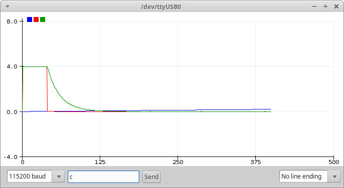
// This system (hardware circuit and software) measures the time
// constant of an RC circuit in order to calculate the value of
// the capacitor. To obtain a time constant of appropriate length,
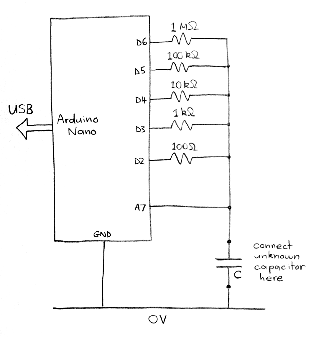
// the system has five resistor values (100, 1k, 10k, 100k, 1M).
// The 100 ohm resistance is only used for charging the capacitor.
// The other four resistances are tried one at a time until a time
// constant longer than 50ms is observed, at which point the
// capacitance is calculated and printed via the Serial Monitor.
//
void setup()
{
pinMode(2, INPUT); // disable 100 ohm resistor
pinMode(3, INPUT); // disable 1k resistor
pinMode(4, INPUT); // disable 10k resistor
pinMode(5, INPUT); // disable 100k resistor
pinMode(6, INPUT); // disable 1M resistor
Serial.begin(115200); // open serial connection
}
void loop()
{
int n; // resistor/pin number, e.g. R3 is 10^3 ohms and on pin D3
float tau, R, C; // time constant, resistance, capacitance
// Try the resistors in this order: 1k, 10k, 100k, 1M.
// The resistance used is equal to 10^n, so the value of n is
// incremented until a time constant over 50ms is observed.
// That time constant is then used to calculate the capacitance.
n = 3;
while (1)
{
tau = measureTimeConstant(n);
if (tau > 50e-3) break;
if (n == 6) break;
if (tau == 0) n = 3; // go back to lowest resistance (1k)
else n++; // move up to higher resistance
}
// Calculate the resistor and capacitor values
R = pow(10,n);
C = tau / R;
// Display the time constant, resistance and capacitance
Serial.print("tau="); Serial.print(1000*tau, 3); Serial.print(" ms, ");
Serial.print("R="); Serial.print(R, 0); Serial.print(" ohm, ");
Serial.print("C=");
if (C < 1e-9) {Serial.print(C*1e12, 3); Serial.print(" pF");}
else if (C < 1e-6) {Serial.print(C*1e9 , 3); Serial.print(" nF");}
else if (C < 1e-3) {Serial.print(C*1e6 , 3); Serial.print(" uF");}
else {Serial.print(C*1e3 , 3); Serial.print(" mF");}
Serial.println();
}
// This function measures the time constant in seconds using resistor n.
float measureTimeConstant(int n)
{
unsigned long t1, t2, timeout;
float Vth;
// Charge the capacitor up to its maximum through the 100 ohm resistor.
pinMode(2, OUTPUT);
digitalWrite(2, HIGH);
delay(1000);
pinMode(2, INPUT);
// Calculate the threshold voltage as 36.8% of the initial voltage.
// The capacitor voltage drops to this value after one time constant.
Vth = 0.36788 * analogRead(7);
// Measure the time constant
t1 = micros(); // record the start time in microseconds
timeout = t1 + 1200000L; // set timeout limit at 1.2 seconds
pinMode(n, OUTPUT); // enable the selected resistor
digitalWrite(n, LOW); // begin discharging the capacitor
while(analogRead(7) > Vth) // wait until voltage drops to Vth (or timeout)
if (micros() > timeout) return 0;
t2 = micros(); // record the end time in microseconds
pinMode(n, INPUT); // disable the selected resistor
return (t2 - t1) * 1e-6; // return the time constant (t2 - t1)
}
The circuit is exactly the same as it was in part 4 of last week’s lab.

This is the circuit on the breadboard. The capacitor near the top left corner of the breadboard is just there as an example. Remove that capacitor before plugging in the wires of your newly built capacitor to measure its capacitance.

Part 2: Construct a simple parallel plate capacitor
To begin with, construct a simple capacitor as follows:
- Cut out two square pieces of aluminium foil, approximately 20 cm x 20 cm, but leaving an extra strip of foil extending from one corner of each piece (for attaching wires).
- Cut two long wires – long enough to reach from the breadboard to opposite corners of your 20 cm x 20 cm square capacitor. Remove the insulation from the last 2 cm of each wire.
- Sellotape one wire onto the corner strip of each piece of foil.

- Lay one piece of foil down smooth flat surface.
- Lay a piece of A4 paper on top of the foil, taking care to cover every part of it except for the strip with the wire attached.
- Lay the second piece of foil down so that it is directly above the first piece (but separated from it by the paper). Orient it so that the corner with the wire attached is not at the same corner as the wire for the lower plate.
- Lay something flat and heavy (like a hardback book) on top to press the three layers tightly together.

- Plug the wires of your capacitor into your breadboard to measure its capacitance. (To give you a rough idea what to expect, when I tried building this capacitor I obtained a capacitance of approximately 15 nF.)
- Try pressing down hard on the stack to squeeze the plates ever closer together. Does it affect the measured capacitance?
- Using the equation from the theory section above, estimate the expected capacitance of this capacitor and compare it to the measured value. When applying the formula, note the following:
- The area of the plates must be expressed in square metres.
- The distance between the plates should be approximately equal to the thickness of the paper sheet. This is difficult to measure directly, but if you measure the height of a stack of sheets then divide by the number of sheets, a reasonably accurate estimate can be obtained. This distance must be expressed in metres.
- Different types of paper will have different relative permittivities. The exact value for the paper you’re using won’t be possible to find, but you should be able to find a reasonable ballpark estimate online.
Retain all your calculations, measurements, and links to information sources so that you can include them all in your lab report next week.
Part 3: Design, build and test a larger capacitor
Now you’re ready to create your own capacitor design, hopefully with a capacitance much greater than that achieved using the simple design described above.
Strategies to consider:
- Increase the area of the plates?
- Try a thinner dielectric material?
- Use a dielectric with a different permittivity?
- Stack more plates together?
- Roll your capacitor into tightly rolled cylinder?
- Create more than one capacitor and combine them in parallel?
Research online to get some more ideas.
Part 4: Write a lab report about the capacitor you built
An example lab report is now available in the Content section of the EEPP2 Brightspace module. The example report is for a different, but closely related, experiment. When you’re ready to write your report, you can use the example report as a template for writing your own account on this experiment. In the meantime, please retain or collect all of the following items:
- Photographs of everything you built, ideally including steps during the build process.
- Screenshots of anything you measured using the capacitance meter (i.e. the Serial Monitor window displaying the measurement).
- Any calculations you carried out. If the calculations were carried out on paper, then retain the written calculations. If the calculations were carried out in MATLAB / Octave, then grab a screenshot or save it to an M-file so that you can refer back to it.
- The sources of any information you obtained online – e.g. material permittivity, thickness of paper / cling film, etc.
 , of an RC circuit is given by the following equation.


 is the instantaneous voltage (in volts) between the terminals of the resistor,
  is the instantaneous current (in amperes) flowing through it, and
  is the resistance (in ohms). This means that at every moment in time, the current flowing through a resistor is proportional to the voltage across it at that instant. This is still true when an AC voltage is applied to a resistor. When you apply a sinusoidal voltage, you get a sinusoidal current with a magnitude that depends on the resistance. The voltage and current waveforms are exactly in phase – i.e. when the voltage is at its peak, the current is also at its peak.
 is the capacitance (in farads). What this means is that the current is proportional to the rate of change of voltage. So when an AC voltage is applied to a capacitor, the magnitude of the current depends on how fast the voltage is changing.
 is the impedance of the resistor (in ohms).
 is the imedance of the capacitor (in ohms),
  is the imaginary unit (i.e.
  ), and
  is the angular frequency (in rad/s). Angular frequency represents the same property of a signal as frequency, but in different units. Whereas frequency is measured in hertz (cycles per second), angular frequency is measured in rad/s (radians per second). When working with impedances, it can be more convenient to use angular frequencies because the arithmetic becomes simpler. Frequency,
  , in hertz and angular frequency,
 (equivalent to
  radians) – i.e. one quarter cycle.


